Appendix B — Python Programming

library(reticulate)

py_install("numpy")
py_install("pandas")
py_install("matplotlib")

import numpy as np
import pandas as pd
import matplotlib.pyplot as plt

B.1 Arithmetic and Logical Operators

2 + 3 / (5 * 4) ** 2

2.0075

5 == 5.00

True

5 == int(5)

True

type(int(5))

<class 'int'>

not True == False

True

bool() converts nonzero numbers to True and zero to False

-5 | 0

-5

1 & 1

bool(2) | bool(0)

True

B.2 Math Functions

Need to import math library in Python.

import math
math.sqrt(144)

12.0

math.exp(1)

2.718281828459045

math.sin(math.pi/2)

1.0

math.log(32, 2)

5.0

abs(-7)

# python comment

B.3 Variables and Assignment

x = 5
x

x = x + 6
x

x == 5

False

math.log(x)

2.3978952727983707

B.4 Object Types

str, float, int and bool.

type(5.0)

<class 'float'>

type(5)

<class 'int'>

type("I_love_data_science!")

<class 'str'>

type(1 > 3)

<class 'bool'>

type(5) is float

False

B.5 Data Structure - Lists

B.5.1 Lists

Python has numbers and strings, but no built-in vector structure.
To create a sequence type of structure, we can use a list that can save several elements in an single object.
To create a list in Python, we use [].

lst_num = [0, 2, 4] 
lst_num

[0, 2, 4]

type(lst_num)

<class 'list'>

len(lst_num)

List elements can have different types!

B.5.2 Subsetting lists

lst = ['data', 'math', 34, True]
lst

['data', 'math', 34, True]

Indexing in Python always starts at 0!
0: the 1st element

lst

['data', 'math', 34, True]

lst[0]

'data'

type(lst[0]) ## not a list

<class 'str'>

-1: the last element

lst[-2]

[a:b]: the (a+1)-th to b-th elements

lst[1:4]

['math', 34, True]

type(lst[1:4]) ## a list

<class 'list'>

[a:]: elements from the (a+1)-th to the last

lst[2:]

[34, True]

What does lst[0:1] return? Is it a list?

B.5.3 Lists are mutable

Lists are changed in place!

lst[1]

'math'

lst[1] = "stats"
lst

['data', 'stats', 34, True]

lst[2:] = [False, 77]
lst

['data', 'stats', False, 77]

If we change any element value in a list, the list itself will be changed as well.

B.5.4 List operations and methods `list.method()`

This is a common syntax in Python. We start with a Python object of some type, then type dot followed by any method specifically for this particular data type or structure for operations.

## Concatenation
lst_num + lst

[0, 2, 4, 'data', 'stats', False, 77]

## Repetition
lst_num * 3

[0, 2, 4, 0, 2, 4, 0, 2, 4]

## Membership
34 in lst

False

## Appends "cat" to lst
lst.append("cat")
lst

['data', 'stats', False, 77, 'cat']

## Removes and returns last object from list
lst.pop()

'cat'

lst

['data', 'stats', False, 77]

## Removes object from list
lst.remove("stats")
lst

['data', False, 77]

## Reverses objects of list in place
lst.reverse()
lst

[77, False, 'data']

B.6 Data Structure - Tuples

Tuples work exactly like lists except they are immutable, i.e., they can’t be changed in place.
To create a tuple, we use ().

tup = ('data', 'math', 34, True)
tup

('data', 'math', 34, True)

type(tup)

<class 'tuple'>

len(tup)

tup[2:]

(34, True)

tup[-2]

tup[1] = "stats"  ## does not work!
# TypeError: 'tuple' object does not support item assignment

tup

('data', 'math', 34, True)

B.6.1 Tuples functions and methods

Lists have more methods than tuples because lists are more flexible.

# Converts a list into tuple
tuple(lst_num)

(0, 2, 4)

# number of occurance of "data"
tup.count("data")

# first index of "data"
tup.index("data")

B.7 Data Structure - Dictionaries

A dictionary consists of key-value pairs.
A dictionary is mutable, i.e., the values can be changed in place and more key-value pairs can be added.
To create a dictionary, we use {"key name": value}.
The value can be accessed by the key in the dictionary.

dic = {'Name': 'Ivy', 'Age': 7, 'Class': 'First'}

dic['Age']

dic['age']  ## does not work

dic['Age'] = 9
dic['Class'] = 'Third'
dic

{'Name': 'Ivy', 'Age': 9, 'Class': 'Third'}

B.7.1 Properties of dictionaries

Python will use the last assignment!

dic1 = {'Name': 'Ivy', 'Age': 7, 'Name': 'Liya'}
dic1['Name']

'Liya'

Keys are unique and immutable.
A key can be a tuple, but CANNOT be a list.

## The first key is a tuple!
dic2 = {('First', 'Last'): 'Ivy Lee', 'Age': 7}
dic2[('First', 'Last')]

'Ivy Lee'

## does not work
dic2 = {['First', 'Last']: 'Ivy Lee', 'Age': 7}
dic2[['First', 'Last']]

B.7.2 Disctionary methods

dic

{'Name': 'Ivy', 'Age': 9, 'Class': 'Third'}

## Returns list of dictionary dict's keys
dic.keys()

dict_keys(['Name', 'Age', 'Class'])

## Returns list of dictionary dict's values
dic.values()

dict_values(['Ivy', 9, 'Third'])

## Returns a list of dict's (key, value) tuple pairs
dic.items()

dict_items([('Name', 'Ivy'), ('Age', 9), ('Class', 'Third')])

## Adds dictionary dic2's key-values pairs in to dic
dic2 = {'Gender': 'female'}
dic.update(dic2)
dic

{'Name': 'Ivy', 'Age': 9, 'Class': 'Third', 'Gender': 'female'}

## Removes all elements of dictionary dict
dic.clear()
dic

{}

B.8 Python Data Structures for Data Science

Python built-in data structures are not specifically for data science.
To use more data science friendly functions and structures, such as array or data frame, Python relies on packages NumPy and pandas.

B.8.1 Installing NumPy and pandas

In your RStudio project, run

library(reticulate)
virtualenv_create("myenv")

Go to Tools > Global Options > Python > Select > Virtual Environments

You may need to restart R session. Do it, and in the new R session, run

library(reticulate)
py_install(c("numpy", "pandas", "matplotlib"))

Run the following Python code, and make sure everything goes well.

import numpy as np
import pandas as pd
v1 = np.array([3, 8])
v1
df = pd.DataFrame({"col": ['red', 'blue', 'green']})
df

B.9 Pandas

pandas is a Python library that provides data structures, manipulation and analysis tools for data science.

import numpy as np
import pandas as pd

B.9.1 Pandas series from a list

# import pandas as pd
a = [1, 7, 2]
s = pd.Series(a)
print(s)

0    1
1    7
2    2
dtype: int64

print(s[0])

## index used as naming 
s = pd.Series(a, index = ["x", "y", "z"])
print(s)

x    1
y    7
z    2
dtype: int64

print(s["y"])

B.9.2 Pandas series from a dictionary

grade = {"math": 99, "stats": 97, "cs": 66}
s = pd.Series(grade)
print(s)

math     99
stats    97
cs       66
dtype: int64

grade = {"math": 99, "stats": 97, "cs": 66}

## index used as subsetting 
s = pd.Series(grade, index = ["stats", "cs"])
print(s)

stats    97
cs       66
dtype: int64

How do we create a named vector in R?

grade <- c("math" = 99, "stats" = 97, "cs" = 66)

B.9.3 Pandas data frame

Create a data frame from a dictionary

data = {"math": [99, 65, 87], "stats": [92, 48, 88], "cs": [50, 88, 94]}

df = pd.DataFrame(data)
print(df)

   math  stats  cs
0    99     92  50
1    65     48  88
2    87     88  94

Row and column names

df.index = ["s1", "s2", "s3"]
df.columns = ["Math", "Stat", "CS"]
df

    Math  Stat  CS
s1    99    92  50
s2    65    48  88
s3    87    88  94

B.9.4 Subsetting columns

In Python, [] returns Series, [[]] returns DataFrame!
In R, [] returns tibble/data frame, [[]] returns vector!

By Names

## Series
df["Math"]

s1    99
s2    65
s3    87
Name: Math, dtype: int64

type(df["Math"])

<class 'pandas.core.series.Series'>

By Index

# ## DataFrame
df[["Math"]]

type(df[["Math"]])

<class 'pandas.core.frame.DataFrame'>

df[["Math", "CS"]]

    Math  CS
s1    99  50
s2    65  88
s3    87  94

isinstance(df[[“Math”]], pd.DataFrame)

B.9.5 Subsetting rows `DataFrame.iloc`

integer-location based indexing for selection by position

df

    Math  Stat  CS
s1    99    92  50
s2    65    48  88
s3    87    88  94

## first row Series
df.iloc[0]

Math    99
Stat    92
CS      50
Name: s1, dtype: int64

## first row DataFrame
df.iloc[[0]]

    Math  Stat  CS
s1    99    92  50

## first 2 rows
df.iloc[[0, 1]]

    Math  Stat  CS
s1    99    92  50
s2    65    48  88

## 1st and 3rd row
df.iloc[[True, False, True]]

    Math  Stat  CS
s1    99    92  50
s3    87    88  94

B.9.6 Subsetting rows and columns `DataFrame.iloc`

df

    Math  Stat  CS
s1    99    92  50
s2    65    48  88
s3    87    88  94

## (1, 3) row and (1, 3) col
df.iloc[[0, 2], [0, 2]]

    Math  CS
s1    99  50
s3    87  94

## all rows and 1st col
df.iloc[:, [True, False, False]]

df.iloc[0:2, 1:3]

    Stat  CS
s1    92  50
s2    48  88

B.9.7 Subsetting rows and columns `DataFrame.loc`

Access a group of rows and columns by label(s)

df

    Math  Stat  CS
s1    99    92  50
s2    65    48  88
s3    87    88  94

df.loc['s1', "CS"]

## all rows and 1st col
df.loc['s1':'s3', [True, False, False]]

df.loc['s2', ['Math', 'Stat']]

Math    65
Stat    48
Name: s2, dtype: int64

B.9.8 Obtaining a single cell value `DataFrame.iat`/ `DataFrame.at`

df

    Math  Stat  CS
s1    99    92  50
s2    65    48  88
s3    87    88  94

df.iat[1, 2]

df.iloc[0].iat[1]

df.at['s2', 'Stat']

df.loc['s1'].at['Stat']

B.9.9 New columns `DataFrame.insert` and new rows `pd.concat`

df

    Math  Stat  CS
s1    99    92  50
s2    65    48  88
s3    87    88  94

df.insert(loc = 2, 
          column = "Chem", 
          value = [77, 89, 76])
df

    Math  Stat  Chem  CS
s1    99    92    77  50
s2    65    48    89  88
s3    87    88    76  94

df1 = pd.DataFrame({
    "Math": 88, 
    "Stat": 99, 
    "Chem": 0, 
    "CS": 100
    }, index = ['s4'])

pd.concat(objs = [df, df1])

    Math  Stat  Chem   CS
s1    99    92    77   50
s2    65    48    89   88
s3    87    88    76   94
s4    88    99     0  100

pd.concat(objs = [df, df1], 
          ignore_index = True)

B.10 NumPy

B.10.1 NumPy for arrays/matrices

NumPy is used to work with arrays/matrices.

The array object in NumPy is called ndarray.
Use array() to create an array.

range(0, 5, 1) # a seq of number from 0 to 4 with increment of 1

range(0, 5)

list(range(0, 5, 1))

[0, 1, 2, 3, 4]

import numpy as np
arr = np.array(range(0, 5, 1)) ## One-dim array 
arr

array([0, 1, 2, 3, 4])

type(arr)

<class 'numpy.ndarray'>

B.10.2 1D array (vector) and 2D array (matrix)

np.arange: Efficient way to create a one-dim array of sequence of numbers

np.arange(2, 5)

array([2, 3, 4])

np.arange(6, 0, -1)

array([6, 5, 4, 3, 2, 1])

2D array

np.array([[1, 2, 3], [4, 5, 6]])

array([[1, 2, 3],
       [4, 5, 6]])

np.array([[[1, 2, 3], [4, 5, 6]], [[1, 2, 3], [4, 5, 6]]])

array([[[1, 2, 3],
        [4, 5, 6]],

       [[1, 2, 3],
        [4, 5, 6]]])

B.10.3 `np.reshape()`

arr2 = np.arange(8).reshape(2, 4)
arr2

array([[0, 1, 2, 3],
       [4, 5, 6, 7]])

arr2.shape

(2, 4)

arr2.ndim

arr2.size

B.10.4 Stacking arrays

a = np.array([1, 2, 3, 4]).reshape(2, 2)
b = np.array([5, 6, 7, 8]).reshape(2, 2)

np.vstack((a, b))

array([[1, 2],
       [3, 4],
       [5, 6],
       [7, 8]])

np.hstack((a, b))

array([[1, 2, 5, 6],
       [3, 4, 7, 8]])

B.11 Plotting

matplotlib.markers

pch = np.array(['.', ',', 'o', 'v', '^', '<', '>', '1', '2', '3', '4', '8', 's', 'p', 'P', '*', 'h', 'H', '+', 'x', 'X', 'D', 'd', '|', '_'])
#all types of maker
pch_len = pch.shape[0]
x = np.array([i for i in range(1, pch_len+1)])
y = np.ones(pch_len)

plt.figure(0)
for i in range(0, pch_len):
    plt.plot(x[i],y[i],pch[i])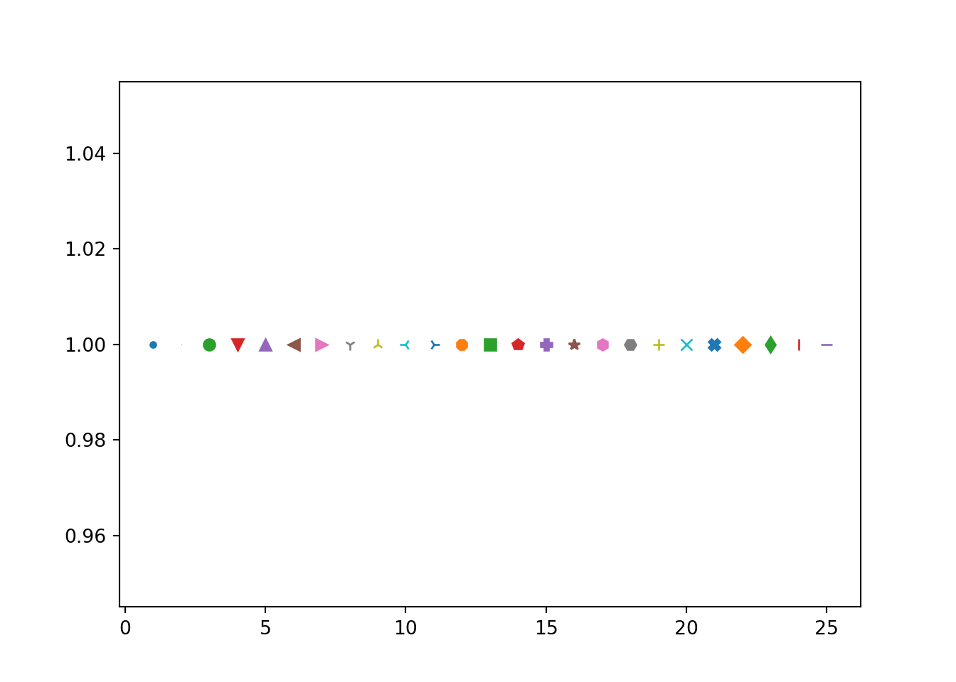

B.11.1 Scatterplot

Code

mtcars = pd.read_csv('./data/mtcars.csv')
mtcars.iloc[0:15,0:4]

     mpg  cyl   disp   hp
0   21.0    6  160.0  110
1   21.0    6  160.0  110
2   22.8    4  108.0   93
3   21.4    6  258.0  110
4   18.7    8  360.0  175
5   18.1    6  225.0  105
6   14.3    8  360.0  245
7   24.4    4  146.7   62
8   22.8    4  140.8   95
9   19.2    6  167.6  123
10  17.8    6  167.6  123
11  16.4    8  275.8  180
12  17.3    8  275.8  180
13  15.2    8  275.8  180
14  10.4    8  472.0  205

import matplotlib.pyplot as plt
plt.scatter(x = mtcars.mpg, y = mtcars.hp, color = "r")
plt.xlabel("Miles per gallon")
plt.ylabel("Horsepower")
plt.title("Scatter plot")

B.11.2 Subplots

The command plt.scatter() is used for creating one single plot. If multiple subplots are wanted in one single call, one can use the format

fig, (ax1, ax2) = plt.subplots(1, 2)
ax1.scatter(x, y)
ax2.plot(x, y)

fig, (ax1, ax2) = plt.subplots(1, 2)
ax1.scatter(x = mtcars.mpg, y = mtcars.hp)
ax2.scatter(x = mtcars.hp, y = mtcars.disp)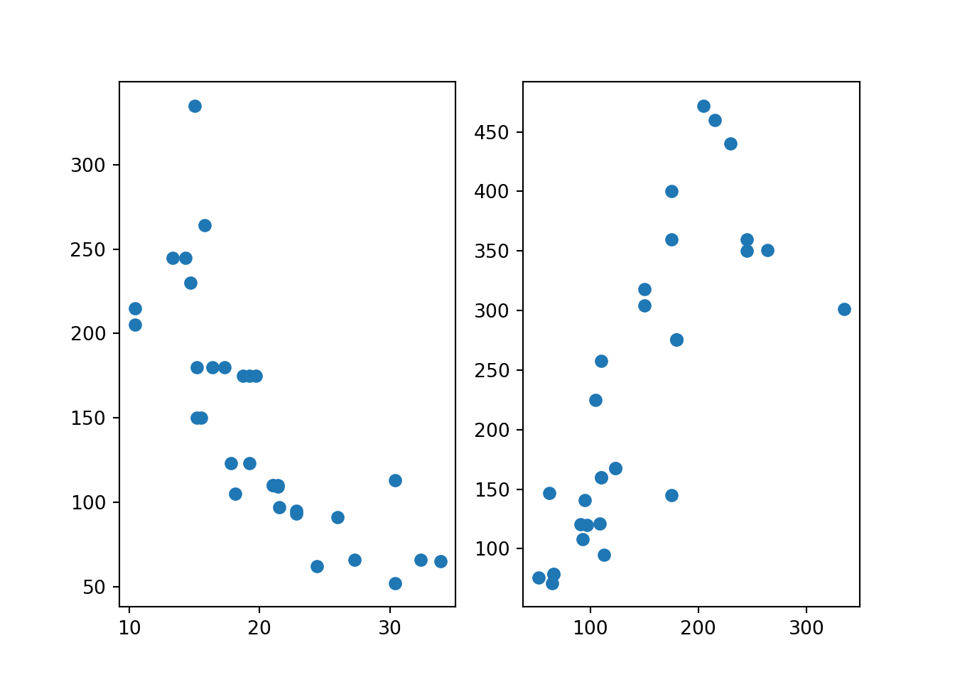

Check Creating multiple subplots using plt.subplots for more details.

B.11.3 Boxplot

Code

cyl_index = np.sort(np.unique(np.array(mtcars.cyl)))
cyl_shape = cyl_index.shape[0]
cyl_list = []
for i in range (0, cyl_shape):
    cyl_list.append(np.array(mtcars[mtcars.cyl == cyl_index[i]].mpg))

plt.boxplot(cyl_list, vert=False, tick_labels=[4, 6, 8])

{'whiskers': [<matplotlib.lines.Line2D object at 0x169998860>, <matplotlib.lines.Line2D object at 0x169998b30>, <matplotlib.lines.Line2D object at 0x169999af0>, <matplotlib.lines.Line2D object at 0x169999dc0>, <matplotlib.lines.Line2D object at 0x16999ac90>, <matplotlib.lines.Line2D object at 0x16999af30>], 'caps': [<matplotlib.lines.Line2D object at 0x169998da0>, <matplotlib.lines.Line2D object at 0x169999040>, <matplotlib.lines.Line2D object at 0x16999a000>, <matplotlib.lines.Line2D object at 0x16999a2d0>, <matplotlib.lines.Line2D object at 0x16999b200>, <matplotlib.lines.Line2D object at 0x16999b4d0>], 'boxes': [<matplotlib.lines.Line2D object at 0x169998740>, <matplotlib.lines.Line2D object at 0x169999820>, <matplotlib.lines.Line2D object at 0x16999aa50>], 'medians': [<matplotlib.lines.Line2D object at 0x169999340>, <matplotlib.lines.Line2D object at 0x16999a540>, <matplotlib.lines.Line2D object at 0x16999b7a0>], 'fliers': [<matplotlib.lines.Line2D object at 0x1699995e0>, <matplotlib.lines.Line2D object at 0x16999a7e0>, <matplotlib.lines.Line2D object at 0x16999ba40>], 'means': []}

plt.xlabel("Miles per gallon")
plt.ylabel("Number of cylinders")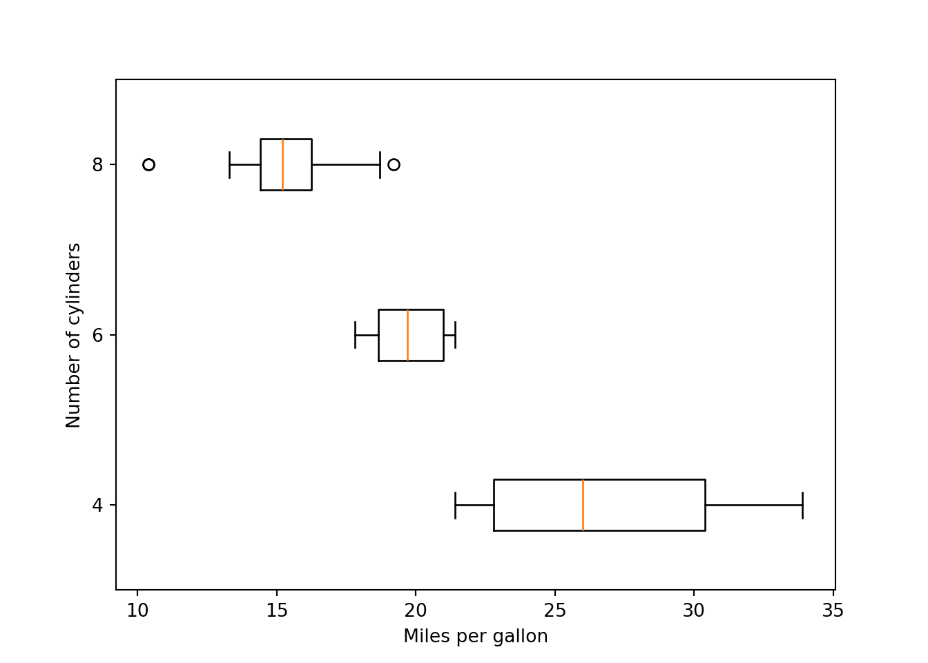

B.11.4 Histogram

plt.hist(mtcars.wt, 
         bins = 19, 
         color="#003366",
         edgecolor="#FFCC00")
plt.xlabel("weights")
plt.title("Histogram of weights")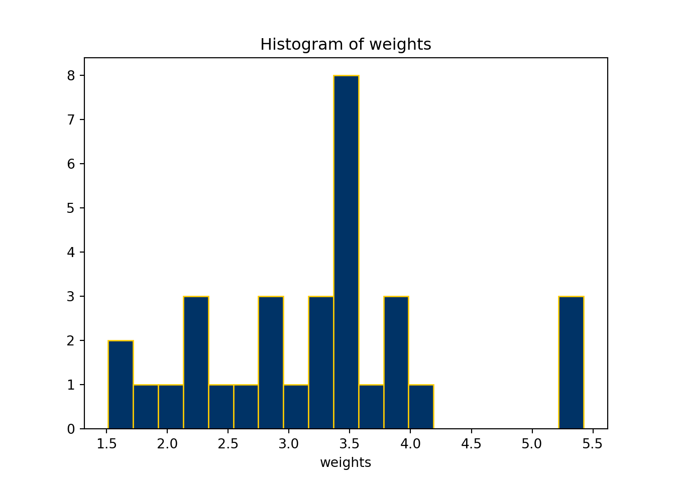

B.11.5 Barplot

count_py = mtcars.value_counts('gear')
count_py

gear
3    15
4    12
5     5
Name: count, dtype: int64

plt.bar(count_py.index, count_py)
plt.xlabel("Number of Gears")
plt.title("Car Distribution")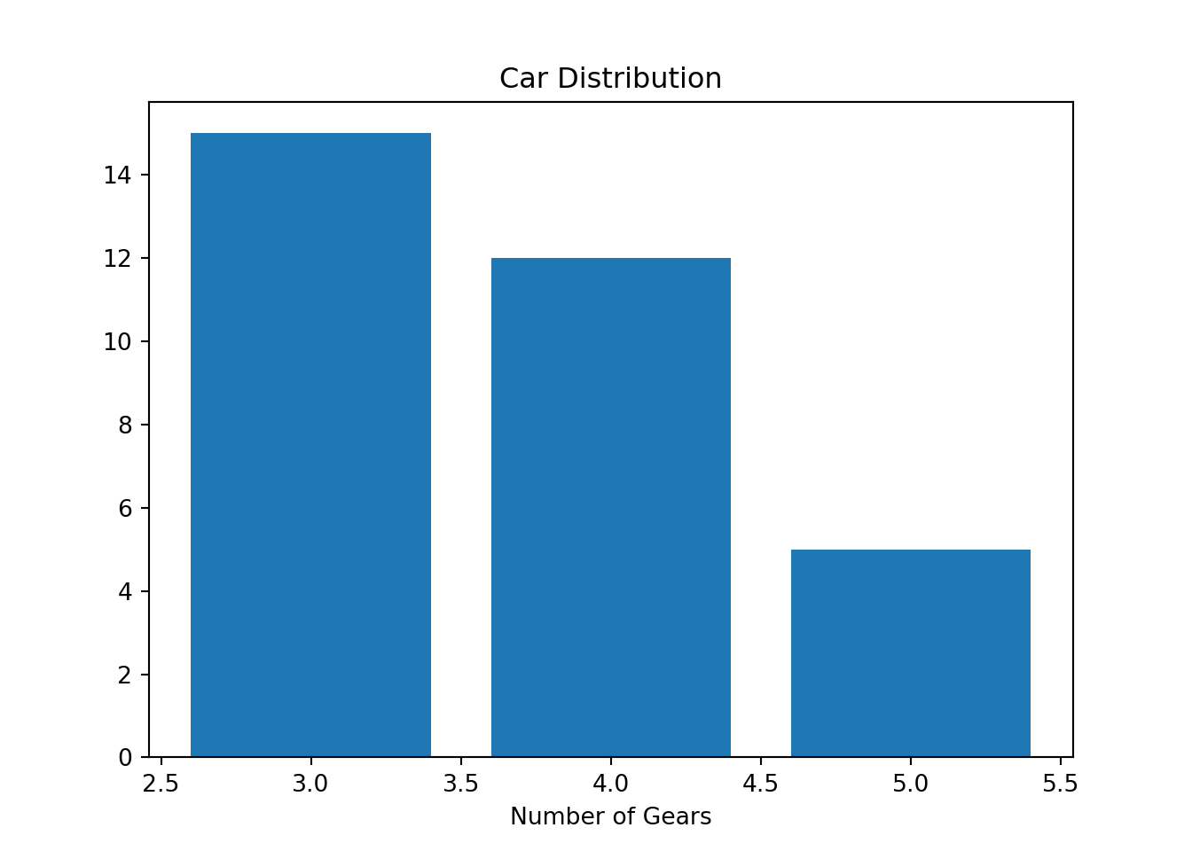

B.11.6 Pie chart

percent = round(count_py / sum(count_py) * 100, 2)
texts = [str(percent.index[k]) + " gear " + str(percent.array[k]) + "%" for k in range(0,3)]

plt.pie(count_py, labels = texts, colors = ['r', 'g', 'b'])

([<matplotlib.patches.Wedge object at 0x16e5bdd90>, <matplotlib.patches.Wedge object at 0x16e5572f0>, <matplotlib.patches.Wedge object at 0x16e5fc320>], [Text(0.10781885436251686, 1.0947031993394165, '3 gear 46.88%'), Text(-0.6111272563215624, -0.9146165735327998, '4 gear 37.5%'), Text(0.9701133907831904, -0.5185364105085978, '5 gear 15.62%')])

plt.title("Pie Charts")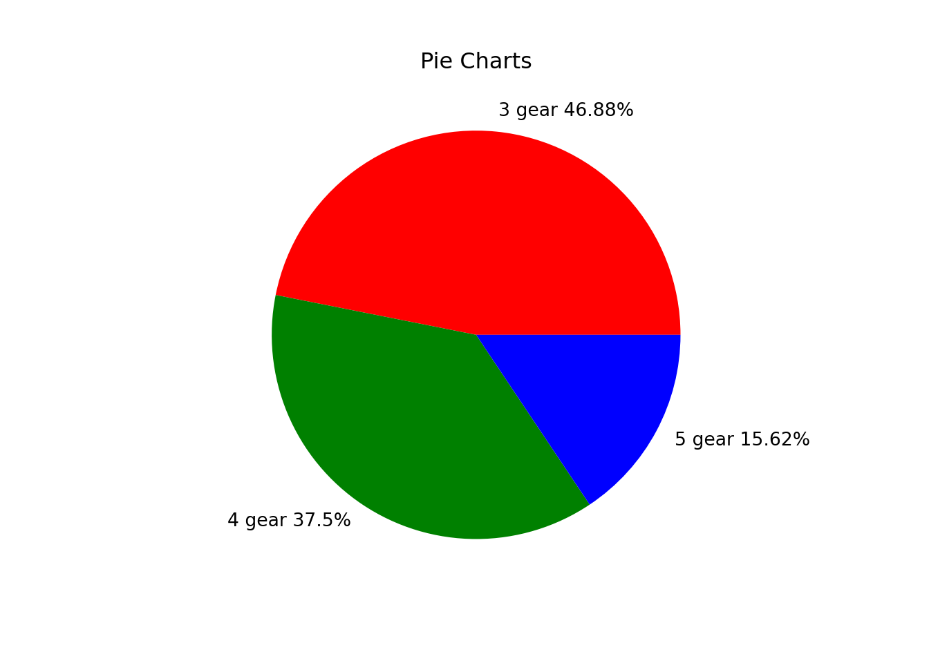

B.11.7 2D Imaging

In Python,

mat_img = np.reshape(np.array(range(1,31)), [6,5], "F")
mat_img

array([[ 1,  7, 13, 19, 25],
       [ 2,  8, 14, 20, 26],
       [ 3,  9, 15, 21, 27],
       [ 4, 10, 16, 22, 28],
       [ 5, 11, 17, 23, 29],
       [ 6, 12, 18, 24, 30]])

plt.imshow(mat_img, cmap = 'Oranges')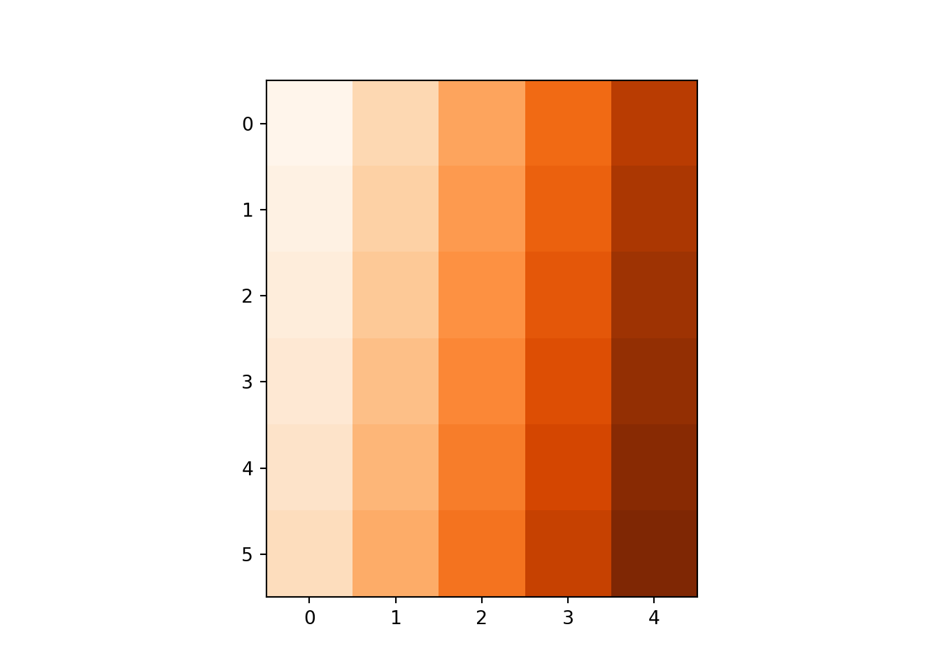

volcano = pd.read_csv('./data/volcano.csv', index_col=0)
x = 10*np.arange(1,volcano.shape[0]+1)
y = 10*np.arange(1,volcano.shape[1]+1)
X,Y = np. meshgrid(x,y)
vt = volcano.transpose()
print(vt.shape)

(61, 87)

print(X.shape)

(61, 87)

print(Y.shape)

(61, 87)

fig, ax = plt.subplots()
IM = ax.matshow(vt, alpha =1, cmap='terrain')
CS = ax.contour(vt, levels=np.arange(90,200,5))
ax.clabel(CS, inline=True, fontsize=10)
ax.set_title('Maunga Whau Volcano')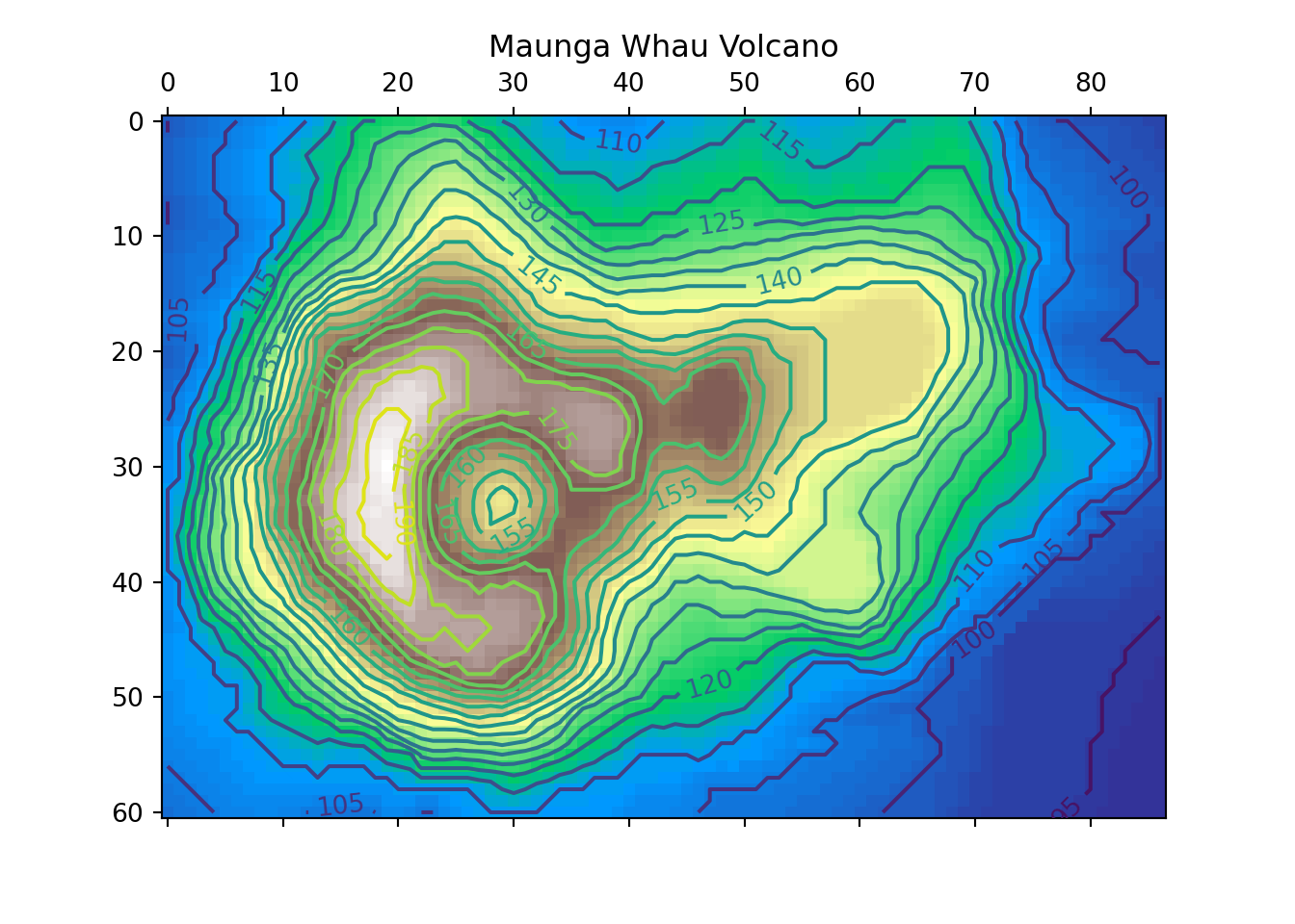

B.11.8 3D scatterplot

In Python,

fig = plt.figure(figsize=(12, 12))
ax = fig.add_subplot(projection='3d')

ax.scatter(xs = mtcars.wt, ys = mtcars.disp, zs = mtcars.mpg)
ax.set_xlabel('Weights')
ax.set_ylabel("Displacement")
ax.set_zlabel("Miles per gallon")
ax.set_title("3D Scatter Plot")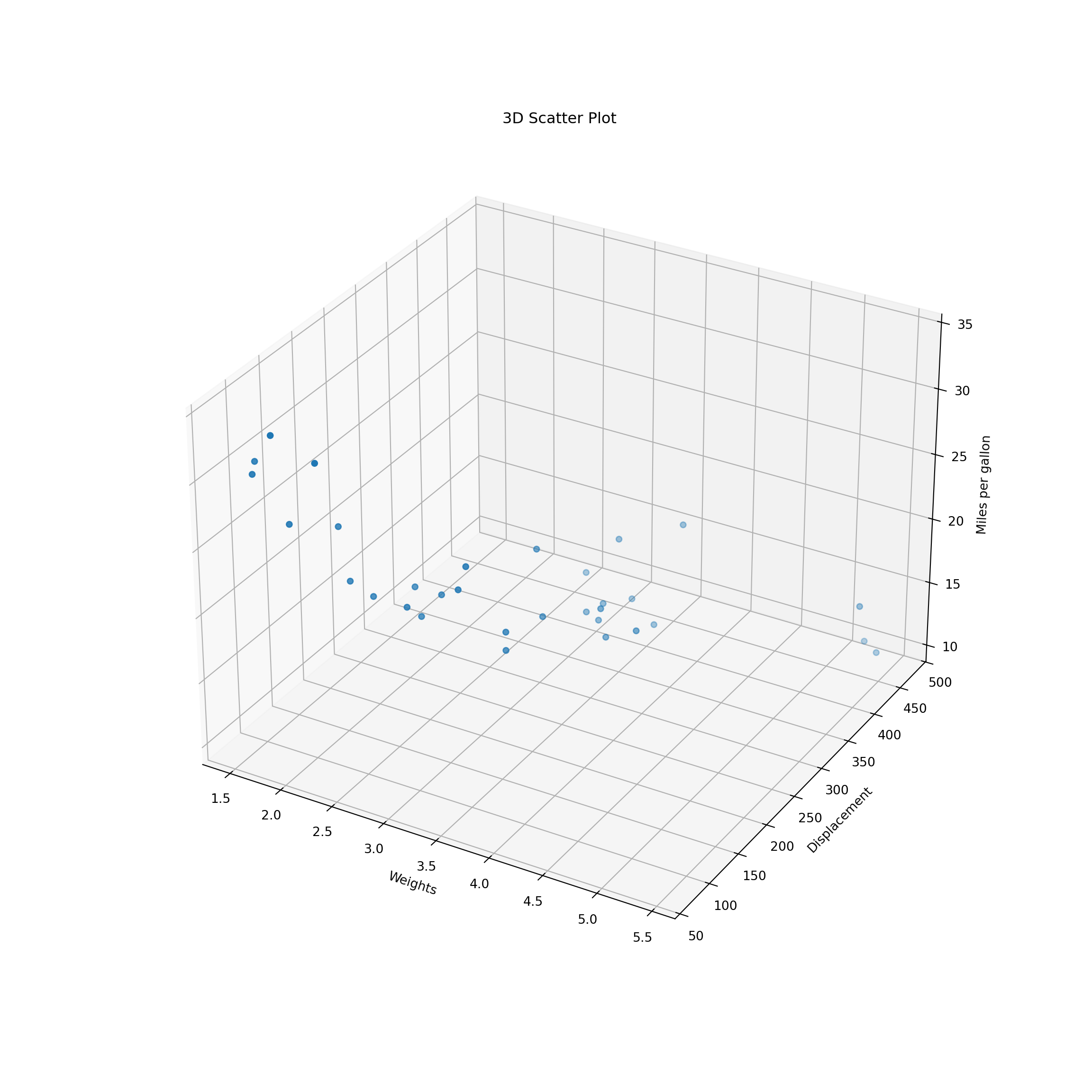

B.11.9 Perspective plot

In Python,

x = 10*np.arange(1,volcano.shape[0]+1)
y = 10*np.arange(1,volcano.shape[1]+1)
vt = volcano.transpose()
Z = 10*vt
X,Y = np. meshgrid(x,y)

print(Z.shape)

(61, 87)

print(X.shape)

(61, 87)

print(Y.shape)

(61, 87)

fig, ax = plt.subplots(subplot_kw={"projection": "3d"})
# Plot the surface.
ax.plot_surface(X, Y, Z, cmap = 'Greens')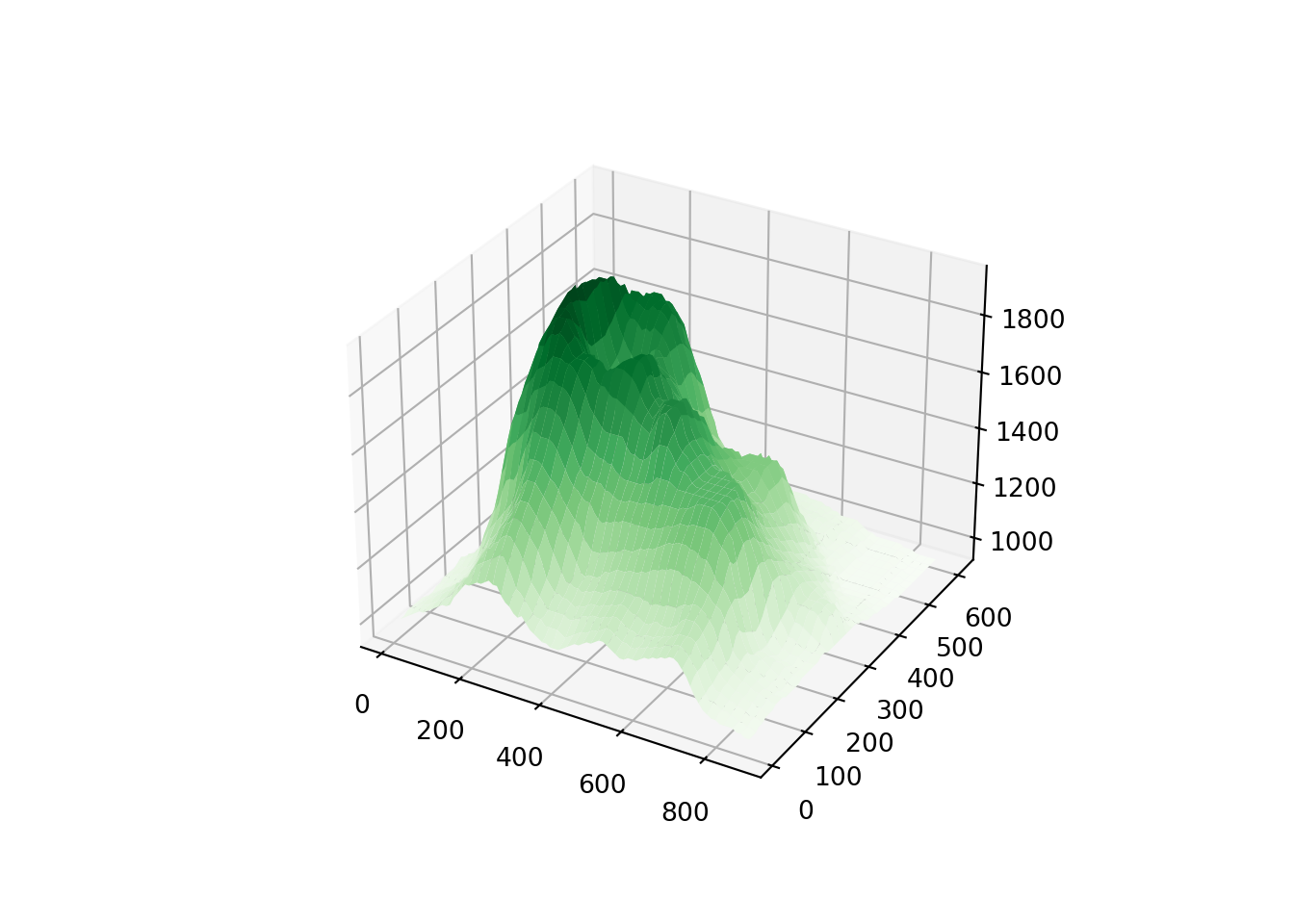

B.12 Special Objects

In python, NA, NaN and NULL are not that distinguishable, comparing to R.

NaN can be used as a numerical value on mathematical operations, while None cannot (or at least shouldn’t).
NaN is a numeric value, as defined in IEEE 754 floating-point standard.
None is an internal Python type (NoneType) and would be more like “inexistent” or “empty” than “numerically invalid” in this context.

a = np.array([None, 0.9, 10])
type(a)

<class 'numpy.ndarray'>

a == None

array([ True, False, False])

len(a)

print(type(a[0]))

<class 'NoneType'>

None == None

True

'' == None

False

a1 = np.array([-1,0,1])/0

<string>:1: RuntimeWarning: divide by zero encountered in divide
<string>:1: RuntimeWarning: invalid value encountered in divide

a1

array([-inf,  nan,  inf])

math.isfinite(0)

True

math.isnan(float("nan"))

True

pd.isna(float("nan"))

True

np.isnan(float("nan"))

True

math.isfinite(7.8/1e-307)

True

math.isfinite(7.8/1e-308)

False

type(None)

<class 'NoneType'>

## TypeError: '>' not supported between instances of 'NoneType' and 'int'
None > 5

## TypeError: object of type 'NoneType' has no len()
len(None)

float("NaN") > 5

False

v_none = np.array([3, None, 5])
v_none

array([3, None, 5], dtype=object)

v_nan = np.array([3, float("NaN"), 5])
v_nan

array([ 3., nan,  5.])

# TypeError: unsupported operand type(s) for +: 'int' and 'NoneType'
sum(v_none)

sum(v_nan)

nan

B.13 Conditions

if condition:
    # code executed when condition is true
else:
    # code executed when condition is false

a = 5
b = 20
if a > 4 or b > 4:
    print('a > 4 or b > 4')

a > 4 or b > 4

if a > 4 and b > 4:
    print('a > 4 and b > 4')

a > 4 and b > 4

if (a > 4) | (b > 4):
    print('a > 4 or b > 4')

a > 4 or b > 4

if (a > 4) & (b > 4):
    print('a > 4 and b > 4')

a > 4 and b > 4

B.14 Multiple conditions

if condition A:
    # do that
elif condition B:
    # do something else
else:
    #

rd = np.random.randint(100)
print(rd)

if rd <= 20:
    print("rd <= 20")
elif rd > 20 and rd <= 40:
    print('rd > 20 and rd <= 40')
elif rd > 40 and rd <= 60:
    print('rd > 40 and rd <= 60')
elif rd > 60 and rd <= 80:
    print('rd > 60 and rd <= 80')
elif rd > 80 and rd <= 100:
    print('rd > 80 and rd <= 100')

rd > 20 and rd <= 40

B.15 Functions

def function_name(arg1, arg2, ...):
    ## body
    return(something)

def add_number(a, b):
    c = a + b
    return c

n1 = 9
n2 = 18
add_number(n1, n2)

B.16 Loops

B.16.1 for loops

Python
for value in that:
    # do this

for i in range(5):
    print('for', i)

for 0
for 1
for 2
for 3
for 4

for i in ['My', '1st', 'for', 'loop']:
    print(i)

My
1st
for
loop

B.16.2 while loops

while (condition):
    # do this

i = 1
while(i < 5):
    print('while',i)
    i = i + 1

while 1
while 2
while 3
while 4

np.random.seed(86)
def flip():
    return np.random.choice(['T','H'], 1)
    
flips = 0
nheads = 0

while(nheads < 3):
    if flip() == "H":
        nheads += 1
    else:
        nheads = 0
    flips += 1
    
flips

B.1 Arithmetic and Logical Operators

B.2 Math Functions

B.3 Variables and Assignment

B.4 Object Types

B.5 Data Structure - Lists

B.5.1 Lists

B.5.2 Subsetting lists

B.5.3 Lists are mutable

B.5.4 List operations and methods list.method()

B.6 Data Structure - Tuples

B.6.1 Tuples functions and methods

B.7 Data Structure - Dictionaries

B.7.1 Properties of dictionaries

B.7.2 Disctionary methods

B.8 Python Data Structures for Data Science

B.8.1 Installing NumPy and pandas

B.9 Pandas

B.9.1 Pandas series from a list

B.9.2 Pandas series from a dictionary

B.9.3 Pandas data frame

B.9.4 Subsetting columns

B.9.5 Subsetting rows DataFrame.iloc

B.9.6 Subsetting rows and columns DataFrame.iloc

B.9.7 Subsetting rows and columns DataFrame.loc

B.9.8 Obtaining a single cell value DataFrame.iat/ DataFrame.at

B.9.9 New columns DataFrame.insert and new rows pd.concat

B.10 NumPy

B.10.1 NumPy for arrays/matrices

B.10.2 1D array (vector) and 2D array (matrix)

B.10.3 np.reshape()

B.10.4 Stacking arrays

B.11 Plotting

B.11.1 Scatterplot

B.11.2 Subplots

B.11.3 Boxplot

B.11.4 Histogram

B.11.5 Barplot

B.11.6 Pie chart

B.11.7 2D Imaging

B.11.8 3D scatterplot

B.11.9 Perspective plot

B.12 Special Objects

B.13 Conditions

B.14 Multiple conditions

B.15 Functions

B.16 Loops

B.16.1 for loops

B.16.2 while loops

B.5.4 List operations and methods `list.method()`

B.9.5 Subsetting rows `DataFrame.iloc`

B.9.6 Subsetting rows and columns `DataFrame.iloc`

B.9.7 Subsetting rows and columns `DataFrame.loc`

B.9.8 Obtaining a single cell value `DataFrame.iat`/ `DataFrame.at`

B.9.9 New columns `DataFrame.insert` and new rows `pd.concat`

B.10.3 `np.reshape()`