25 Multiple Comparison*

25.1 Multiplicity of Hypotheses

What do we do after ANOVA? In ANOVA we test

$\begin{aligned} H_{0} : μ_{1} = μ_{2} = \dots = μ_{t} \\ H_{1} : μ_{i} \neq μ_{j} for some i, j \end{aligned}$

If we reject $H_{0}$ in favor of $H_{1}$ , we conclude that at least one of the $t$ population means differ from the others, or $μ_{i} \neq μ_{j}$ for some $i$ and $j$ . But the question is, we only conclude that there is some difference, but we don’t know which means differ from each other, or what pairs $(μ_{i}, μ_{j})$ are different. ANONA itself does not answer such questions. Results of an ANOVA do NOT tell us which group(s) is(are) different from the others.

So after ANOVA, we may want to test

$\begin{aligned} H_{0}^{i j} : μ_{i} = μ_{j} \\ H_{1}^{i j} : μ_{i} \neq μ_{j} \end{aligned}$ for all pairs of $(i, j)$ using, say, two-sample $t$ -test.

We will be testing many hypotheses. As we discussed before, if there are $t$ populations under the study, there are $t$ chooses 2 $(\binom{t}{2})$ pairs to be tested. For example, if there are 5 treatments, there will be 10 hypotheses. The test statistic will be like $t_{i j} = \frac{{\bar{y}}_{i} - {\bar{y}}_{j}}{s_{p}^{i j} \sqrt{(\frac{1}{n_{i}} + \frac{1}{n_{j}})}}$ for all pairs of $(i, j)$ , assuming all have the same population variance.

However, performing too many pairewise tests simultaneously is problematic. If there are 10 hypotheses and each is tested at $α = 0.05$ , there will be a high chance that one hypothesis will be falsely rejected. $\begin{aligned} P (At least 1 hypothesis is falsely rejected) & = 1 - P (No hypothesis is falsely rejected) \\ = 1 - (1 - α)^{t} \\ = 1 - (1 - 0.05)^{10} = 0.4 \end{aligned}$ provided that all tests or hypotheses are independent. This probability is called the family-wise error rate (FWER). We’ll take about it in more detail later.

This high probability problem always arises due to multiplicity of hypotheses, meaning that multiple testings are conducted simultaneously in one single research study. This problem of multiplicity is more serious when you are testing more hypotheses.

[Example: Gene Expression Analysis] A data set is collected on gene expressions on 10,000 genes. This kind of research is done if you are trying to find genes responsible for cancer. If those genes are correctly detected, you can study their structure and come up with a cure.

If we test each of the hypotheses at $α = 0.05$ , then $P (At least 1 hypothesis is falsely rejected) \approx 1$ . In fact, on average 5% of them (500 hypotheses) will be falsely discovered even if all null hypotheses are true. This is a big problem in scientific studies.

In this chapter we will learn how to do multiple pairwise comparisons or testings simultaneously while controlling the familywise error rate at a low level, reducing the number of false positives, or mitigating the inflated Type-I error rate due to multiple comparisons. The main methods introduced here include Bonferroni correction, Fisher’s LSD (Least Significant Difference), Tukey’s HSD (honestly significant difference), and Dunnett’s Method. Before we jump into these methods, let’s first look at an examples, refreshing our knowledge of ANOVA.

Example of Multiple Comparison: ANOVA (Example 9.4 in SMD)

A study was done to test 5 different agents used to control weeds. Each of these agents were applied to sample of 6 one-acre plots. The hay was harvested and the total yield was recorded.

R
Python

The data set is saved in the R data frame data_weed.

   yield agent type
1   1.05     1 None
2   1.09     1 None
3   1.32     1 None
4   1.13     1 None
5   1.13     1 None
6   1.33     1 None
7   1.37     2 Bio1
8   1.12     2 Bio1
9   1.20     2 Bio1
10  1.24     2 Bio1
11  1.47     2 Bio1
12  1.35     2 Bio1
13  1.36     3 Bio2
14  1.33     3 Bio2
15  1.27     3 Bio2
16  1.50     3 Bio2
17  1.37     3 Bio2
18  1.14     3 Bio2
19  1.64     4 Chm1
20  1.41     4 Chm1
21  1.30     4 Chm1
22  1.46     4 Chm1
23  1.31     4 Chm1
24  1.37     4 Chm1
25  1.45     5 Chm2
26  1.34     5 Chm2
27  1.61     5 Chm2
28  1.54     5 Chm2
29  1.40     5 Chm2
30  1.66     5 Chm2

Summary statistics are shown below.

 agent sample_mean sample_sd sample_size type
     1        1.17     0.120           6 None
     2        1.29     0.127           6 Bio1
     3        1.33     0.120           6 Bio2
     4        1.42     0.125           6 Chm1
     5        1.50     0.127           6 Chm2

The data set is saved in the Python data frame data_weed.

import pandas as pd
# Load the data from a CSV file
data_weed = pd.read_csv("./data/data_weed.csv")
data_weed

     yield  agent  type
0   1.0480      1   NaN
1   1.0896      1   NaN
2   1.3151      1   NaN
3   1.1275      1   NaN
4   1.1349      1   NaN
5   1.3348      1   NaN
6   1.3659      2  Bio1
7   1.1238      2  Bio1
8   1.2049      2  Bio1
9   1.2387      2  Bio1
10  1.4730      2  Bio1
11  1.3517      2  Bio1
12  1.3621      3  Bio2
13  1.3342      3  Bio2
14  1.2703      3  Bio2
15  1.4950      3  Bio2
16  1.3714      3  Bio2
17  1.1350      3  Bio2
18  1.6369      4  Chm1
19  1.4142      4  Chm1
20  1.3014      4  Chm1
21  1.4625      4  Chm1
22  1.3093      4  Chm1
23  1.3657      4  Chm1
24  1.4532      5  Chm2
25  1.3362      5  Chm2
26  1.6145      5  Chm2
27  1.5390      5  Chm2
28  1.3967      5  Chm2
29  1.6603      5  Chm2

 agent sample_mean sample_sd sample_size type
     1        1.17     0.120           6 None
     2        1.29     0.127           6 Bio1
     3        1.33     0.120           6 Bio2
     4        1.42     0.125           6 Chm1
     5        1.50     0.127           6 Chm2

The questions are

if there is a difference between the agents
which agent provides the best yield

The first question can be answered by ANOVA. Let’s check the assumptions, and perform ANOVA.

First we check the equality of variances $H_{0} : σ_{1}^{2} = \dots = σ_{5}^{2}$ .

R
Python

library(car)
(levene_test <- leveneTest(yield ~ agent, data = data_weed))

Levene's Test for Homogeneity of Variance (center = median)
      Df F value Pr(>F)
group  4    0.12   0.97
      25

# Bartlett test is adapted for normally distributed data.
(bartlett_test <- bartlett.test(yield ~ agent, data = data_weed))


    Bartlett test of homogeneity of variances

data:  yield by agent
Bartlett's K-squared = 0.03, df = 4, p-value = 1

# The Fligner-Killeen test is most robust against departures from normality. Use it when there are outliers.
(fligner_test <- fligner.test(yield ~ agent, data = data_weed))


    Fligner-Killeen test of homogeneity of variances

data:  yield by agent
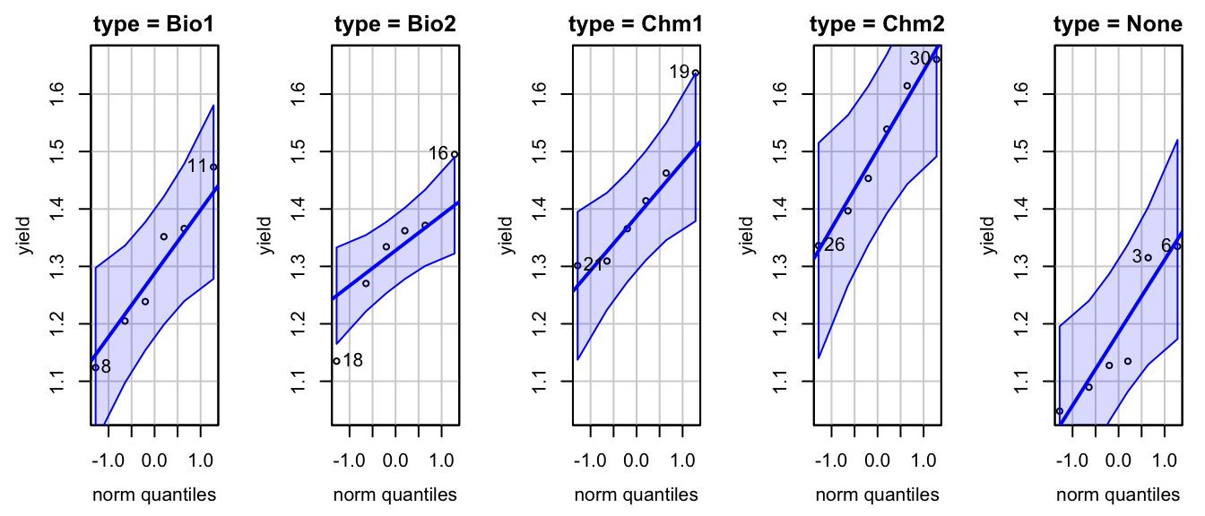
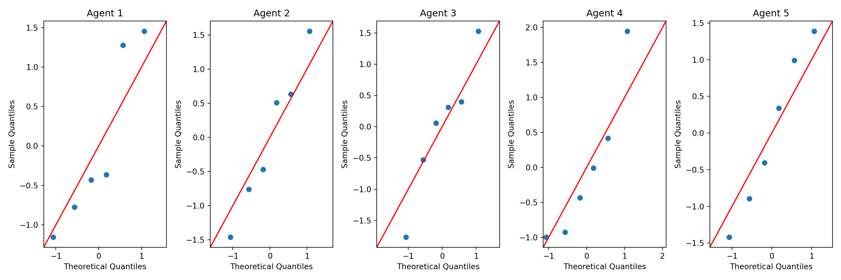
Fligner-Killeen:med chi-squared = 0.4, df = 4, p-value = 1

Then we check the normality assumption $H_{0} :$ Data are generated from a normal distribution for each type of weed agents. The qqplot looks good.

library(car)
qqPlot(yield ~ type, data = data_weed, layout=c(1, 5))

import scipy.stats as stats
import statsmodels.api as sm
from statsmodels.formula.api import ols

# Levene's Test
# https://docs.scipy.org/doc/scipy/reference/generated/scipy.stats.levene.html
stats.levene(data_weed['yield'][data_weed['agent'] == 1],
             data_weed['yield'][data_weed['agent'] == 2],
             data_weed['yield'][data_weed['agent'] == 3],
             data_weed['yield'][data_weed['agent'] == 4],
             data_weed['yield'][data_weed['agent'] == 5])

LeveneResult(statistic=0.11984660886763815, pvalue=0.9741358089178117)

# Bartlett's Test 
# https://docs.scipy.org/doc/scipy/reference/generated/scipy.stats.bartlett.html
stats.bartlett(data_weed['yield'][data_weed['agent'] == 1],
               data_weed['yield'][data_weed['agent'] == 2],
               data_weed['yield'][data_weed['agent'] == 3],
               data_weed['yield'][data_weed['agent'] == 4],
               data_weed['yield'][data_weed['agent'] == 5])

BartlettResult(statistic=0.02859647293854971, pvalue=0.99989874938744)

# Fligner-Killeen Test
# https://docs.scipy.org/doc/scipy/reference/generated/scipy.stats.fligner.html
stats.fligner(data_weed['yield'][data_weed['agent'] == 1],
              data_weed['yield'][data_weed['agent'] == 2],
              data_weed['yield'][data_weed['agent'] == 3],
              data_weed['yield'][data_weed['agent'] == 4],
              data_weed['yield'][data_weed['agent'] == 5])

FlignerResult(statistic=0.4334833327653211, pvalue=0.9796448746915967)

Then we check the normality assumption $H_{0} :$ Data are generated from a normal distribution for each type of weed agents. The qqplot looks good.

Next, we perform ANOVA to test if there is a difference among the agents.

$\begin{aligned} H_{0} : μ_{1} = μ_{2} = \dots = μ_{5} \\ H_{1} : μ_{i} \neq μ_{j} for some pairs (i, j) \end{aligned}$

R
Python

anova(lm(yield ~ agent, data = data_weed))

Analysis of Variance Table

Response: yield
          Df Sum Sq Mean Sq F value Pr(>F)   
agent      4  0.365  0.0912    5.96 0.0016 **
Residuals 25  0.383  0.0153                  
---
Signif. codes:  0 '***' 0.001 '**' 0.01 '*' 0.05 '.' 0.1 ' ' 1

## need to rename yield. need to figure out why
data_weed.rename(columns={'yield': 'yield_value'}, inplace=True)
sm.stats.anova_lm(ols('yield_value ~ C(agent)', data=data_weed).fit())

            df    sum_sq   mean_sq         F    PR(>F)
C(agent)   4.0  0.364675  0.091169  5.958351  0.001647
Residual  25.0  0.382525  0.015301       NaN       NaN

We reject $H_{0}$ , and conclude that there is a difference among the agents.

In the ANOVA, we only conclude that mean yields are different under different agents. How do we say which agent is the best? Are chemical agents (Agent 4, 5) better than the biological agents (Agent 2, 3)? All of these questions can be answered by all pairwise comparisons.

$\begin{aligned} H_{0}^{i j} : μ_{i} = μ_{j} \\ H_{1}^{i j} : μ_{i} \neq μ_{j} \end{aligned}$

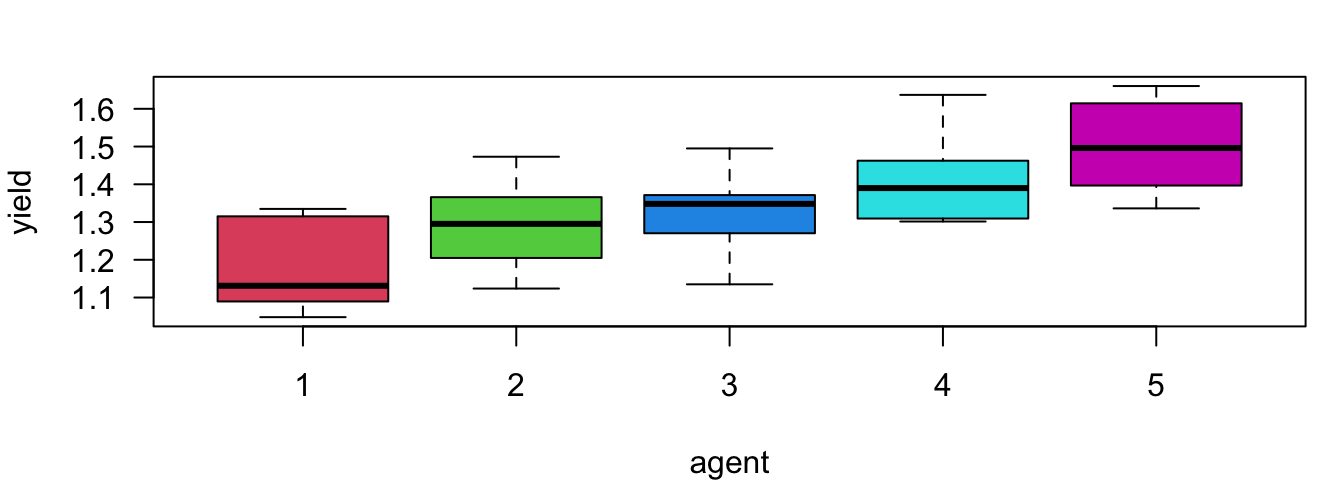
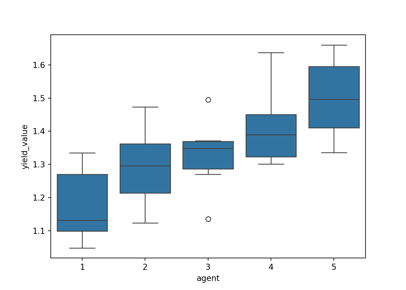
Here shows the boxplot for each weed agent. The ANOVA has told us there are some mean yield differences among these agents, and we are going to find out which 2 agents or which pair produce statistically discernible different mean yields.

R
Python

25.2 Familywise Error Rate (FWER) and Bonferroni Correction

25.2.1 Familywise Error Rate (FWER)

Instead of using Type I error rate $α$ for each single 2-sample test, we should use a different type of error rate. We need to control the so-called familywise error rate (FWER) denoted as $α_{F} = P (Falsely reject at least one hypotheses) \leq α_{0}$ , $F$ for Familywise. This is a probability of falsely rejecting at least one hypothesis of all the hypotheses considered. We hope $α_{F}$ is less than or equal to some small value say $α_{0}$ , just like we hope the Type I error rate of each individual test $α < 0.05$ .

The idea is that when we are doing multiple comparisons, we view all the comparisons, here in the weed yield example, all 10 2-sample tests, as a whole single problem like one single family, and we are controlling the falsely rejection rate for that one family, not the falsely rejection rate for every single family member, a 2 sample test in the family.

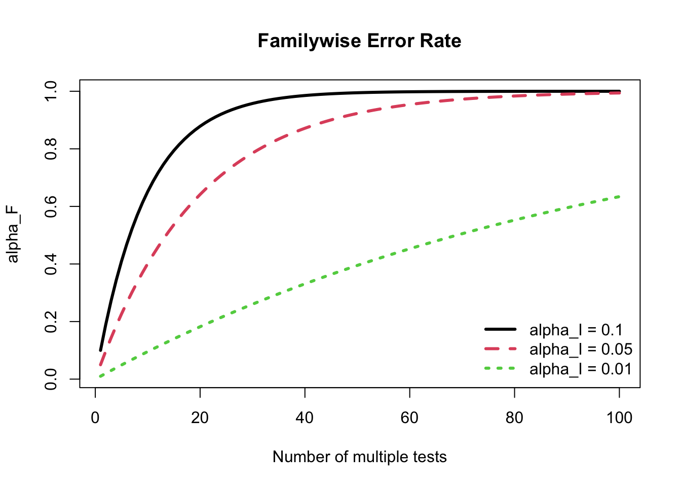
If there are $m$ (independent) hypotheses each tested at significance level $α_{I}$ , then $α_{F} = 1 - (1 - α_{I})^{m}$ . So the larger $m$ is, the higher $α_{F}$ is. To achieve a desired level of $α_{F}$ , which is typically as small as individual $α_{I}$ , we might lose power of true discovery because to make $α_{F}$ small, that is, we decrease the probability of falsely rejecting a $H_{0}$ , we tend to be more conservative to reject $H_{0}$ , and we make it harder to reject $H_{0}$ . But when doing so, we may miss some false $H_{0}$ that should have been rejected.

As shown in the figure below, if $α_{I} = 0.1$ , then $α_{F} \approx 1$ when $m$ is more than 40, meaning that there will definitely be a false discovery in the study. If $α_{I} = 0.05$ , then the probability of committing a false discovery is higher than 80%! In practice, $m$ can be 10 thousands or even millions large. Then $α_{F}$ is basically one, and there are lots of false rejections of $H_{0}$ in the study, resulting in misleading scientific conclusions. We need to find a way to control or adjust $α_{F}$ to a much smaller level.

25.2.2 Bonferroni Correction

We will discuss four methods: Bonferroni, Fisher’s LSD (Least Significant Difference), Tukey’s HSD (Honestly Significant Difference), and Dunnett’s method. With $H_{0}^{i j} : μ_{i} = μ_{j}$ and $H_{1}^{i j} : μ_{i} \neq μ_{j}$ , in all of the methods we reject $H_{0}^{i j}$ if $| {\overset{―}{y}}_{i} - {\overset{―}{y}}_{j} | > C$ for some value $C$ .

The idea is that when $μ_{i} \neq μ_{j}$ , it’s more likely to have large $| {\overset{―}{y}}_{i} - {\overset{―}{y}}_{j} |$ . When $| {\overset{―}{y}}_{i} - {\overset{―}{y}}_{j} |$ is so large that is over some determined threshold $C$ , we conclude that $μ_{i} \neq μ_{j}$ . Think about the 2-sample pooled $t$ -test. The test statistic is $t_{t e s t} = \frac{{\overset{―}{y}}_{1} - {\overset{―}{y}}_{2}}{\sqrt{s_{p}^{2} (\frac{1}{n_{1}} + \frac{1}{n_{2}})}}$ , and we reject $H_{0}$ if $| t_{t e s t} | > t_{α / 2, n_{1} + n_{2} - 2}$ . Therefore, we reject $H_{0}$ if

$| {\overset{―}{y}}_{1} - {\overset{―}{y}}_{2} | > t_{α / 2, n_{1} + n_{2} - 2} \sqrt{s_{p}^{2} (\frac{1}{n_{1}} + \frac{1}{n_{2}})} .$

The problem is the threshold $t_{α / 2, n_{1} + n_{2} - 2} \sqrt{s_{p}^{2} (\frac{1}{n_{1}} + \frac{1}{n_{2}})}$ is not that good when lots of tests being considered simultaneously. The multiple comparison methods try to provide better critical value and estimate of variance, so that $α_{F}$ is properly controlled. We will look into the pros and cons for these methods later.

The first method is Bonferroni correction. The Bonferroni inequality provides a method for selecting $α_{I}$ so that $α_{F}$ is bounded below a specific value. The Bonferroni inequality provides a rough upper bound for $α_{F}$ that $α_{F} = 1 - (1 - α_{I})^{m} \leq (α_{I}^{0} + \dots + α_{I}^{m}) .$ When each of the $m$ tests has the same rate $α_{I}$ , $α_{F} \leq m α_{I} .$

If there are $m$ hypotheses, and we want $α_{F} \leq α_{0} = 0.05$ , then we can test individual hypothesis at $α_{I} = \frac{α_{0}}{m} = \frac{0.05}{m}$ , and then use a standard method such as $t$ -test. This will guarantee that $α_{F} \leq m α_{I} = m (\frac{α_{0}}{m}) = m (\frac{0.05}{m}) = 0.05 .$

However, the problem with this approach is that if $m$ is large, $α_{I} = \frac{0.05}{m}$ will be very small, and the chance of rejecting $H_{0}$ will be small. This correction procedure is very conservative with respect to $α_{F}$ and the power of Bonferroni correction method is very poor.

In the Bonferroni method, we use test statistic $t_{i j} = \frac{| {\overset{―}{y}}_{i} - {\overset{―}{y}}_{j} |}{\sqrt{{\hat{σ}}^{2} (\frac{1}{n_{i}} + \frac{1}{n_{j}})}}$ with Type I error rate of $α_{I} = \frac{α}{m}$ , $m$ is the number of hypotheses.

The value ${\hat{σ}}^{2} = s_{W}^{2} = M S W = \frac{S S W}{d f_{W}}$ from ANOVA is the pooled variance (pooled by total $t$ samples) that estimates the common variance $σ^{2}$ , where $d f_{W} = n_{1} + \dots + n_{t} - t$ . We then reject $H_{0}$ or say that pair $(μ_{i}, μ_{j})$ are statistically discernibly different if $| {\overset{―}{y}}_{i} - {\overset{―}{y}}_{j} | > t_{\frac{α}{2 m}, d f_{W}} \sqrt{s_{W}^{2} (\frac{1}{n_{i}} + \frac{1}{n_{j}})}$

Look at the formula carefully. The differences between Bonferroni and the unadjusted 2-sample pooled $t$ -test are

Change the critical value from $t_{\frac{α}{2}, n_{i} + n_{j} - 2}$ to $t_{\frac{α / m}{2}, n_{1} + \dots + n_{t} - t}$
Change the pooled variance from $s_{p}^{2}$ pooled by the $i$ -th and $j$ -th samples only to ${\hat{σ}}^{2} = s_{W}^{2}$ pooled by all $t$ samples

In Bonferroni method, we make the individual error rate smaller, and we consider all groups when estimating $σ^{2}$ . The estimate ${\hat{σ}}^{2}$ is generally better than $s_{p}^{2}$ because it averages over more sample variances together, and it makes the estimate less varied and closer to the true value of $σ^{2}$ if the truth is that all populations have the common $σ^{2}$ . Think about it. ${\hat{σ}}^{2}$ uses more information from all samples, but $s_{p}^{2}$ only considers the $i$ th and $j$ th groups.

Example of Multiple Comparison: Bonferroni

 agent sample_mean sample_sd sample_size type
     1        1.17     0.120           6 None
     2        1.29     0.127           6 Bio1
     3        1.33     0.120           6 Bio2
     4        1.42     0.125           6 Chm1
     5        1.50     0.127           6 Chm2

Back to the weed yield example, and see the pair comparison result using the Bonferroni method. We have 5 different weed agents. One is control group, no agent (Agent 1), 2 biological agents (Agent 2 and 3), and 2 chemical agents (Agent 4 and 5).

We know $n_{i}$ and $s_{i}$ , so we can get the followings:

$S S W = \sum_{i} (n_{i} - 1) s_{i}^{2} = 0.3825$ , $d f_{W} = 25$ .
$s_{W}^{2} = M S W = {\hat{σ}}^{2} = \frac{S S W}{d f_{W}} = \frac{0.3825}{25} = 0.0153$ .

Also, set $α = 0.05$ , and $m = 10$ , so

$\frac{α}{2 m} = \frac{0.05}{2 \cdot 10} = 0.0025$ , and $t_{\frac{α}{2 m} = 0.0025, d f_{W} = 25} = 3.078$

Therefore, using the Bonferroni method, we conclude $μ_{i} - μ_{j} \neq 0$ if $| {\overset{―}{y}}_{i} - {\overset{―}{y}}_{j} | > 3.078 \sqrt{0.0153 (\frac{1}{6} + \frac{1}{6})} = 0.2198 .$

Here lists comparisons between Agent 1 (control) with Agent 2 to 5.

Agent 1 v.s. 5: $| 1.500 - 1.175 | = 0.325 > 0.2198$
Agent 1 v.s. 4: $| 1.415 - 1.175 | = 0.240 > 0.2198$
Agent 1 v.s. 3: $| 1.328 - 1.175 | = 0.153 < 0.2198$
Agent 1 v.s. 2: $| 1.293 - 1.175 | = 0.118 < 0.2198$

We can see that Chm2 (Agent 5) and Chm1 (Agent 4) are different from Control (Agent 1), but Bio1 and Bio2 are not significantly different from the control group.

$| {\overset{―}{y}}_{i} - {\overset{―}{y}}_{j} | > t_{\frac{α}{2 m}, d f_{W}} \sqrt{s_{W}^{2} (\frac{1}{n_{i}} + \frac{1}{n_{j}})}$

R
Python

Let me first show how I do the Bonferroni correction using R step by step.

y_bar <- c(1.175, 1.293, 1.328, 1.415, 1.500)
## all pairs
(y_bar_pair <- combn(y_bar, 2))

     [,1] [,2] [,3] [,4] [,5] [,6] [,7] [,8] [,9] [,10]
[1,] 1.18 1.18 1.18 1.18 1.29 1.29 1.29 1.33 1.33  1.42
[2,] 1.29 1.33 1.42 1.50 1.33 1.42 1.50 1.42 1.50  1.50

## all pair distances |y_bar_i - y_bar_j|
y_bar_dist <- apply(y_bar_pair, 2, dist)
dd <- t(combn(1:5, 2))
names(y_bar_dist) <- paste(dd[, 1], dd[, 2], sep = " vs ")
y_bar_dist

1 vs 2 1 vs 3 1 vs 4 1 vs 5 2 vs 3 2 vs 4 2 vs 5 3 vs 4 3 vs 5 4 vs 5 
 0.118  0.153  0.240  0.325  0.035  0.122  0.207  0.087  0.172  0.085

## set values
alpha <- 0.05; m <- choose(5, 2); n <- 6

## perform anova
aov_res <- aov(yield ~ agent, data = data_weed) 

## extract df_W
(df <- df.residual(aov_res))

[1] 25

## extract s_W
(sw <- sigma(aov_res) )

[1] 0.124

## critical value of bonferroni
(t_bon <- qt(p = alpha / (2 * m), df = df, lower.tail = FALSE))

[1] 3.08

## margin of error
(E_bon <- t_bon * sw * sqrt((1/n + 1/n)))

[1] 0.22

## decision
(y_bar_dist > E_bon)

1 vs 2 1 vs 3 1 vs 4 1 vs 5 2 vs 3 2 vs 4 2 vs 5 3 vs 4 3 vs 5 4 vs 5 
 FALSE  FALSE   TRUE   TRUE  FALSE  FALSE  FALSE  FALSE  FALSE  FALSE

There is a shortcut to do Bonferroni correction for pairwise comparisons. We can use the function pairwise.t.test(). If we want to do 2-sample pooled $t$ test, argument pool.sd should be FALSE because this argument is for the pooled variance pooled by all groups combined, not group $i$ and $j$ . The p.adjust.method is none because we do not control or adjust FWER. The var.equal should be TRUE, so that the pooled $t$ test is used. Otherwise, it will perform 2 sample $t$ test with non-equal variances.

The output is a matrix including p-values of all pair comparison testings. We can tell which pairs are significant by comparing their p-value with the significance level $α$ .

If we want to do Bonferroni correction, use p.adjust.method = "bonferroni". Again, in Bonferroni, (1, 4) and (1, 5) are statistically significantly different. In traditional 2 sample $t$ test, significant results include (1, 4), (1, 5), (2, 5), and (3, 5).

## individual 2-sample pooled t-test but not pooled by all groups
pairwise.t.test(data_weed$yield, data_weed$agent, pool.sd = FALSE,
                p.adjust.method = "none", var.equal = TRUE)


    Pairwise comparisons using t tests with non-pooled SD 

data:  data_weed$yield and data_weed$agent 

  1     2     3     4    
2 0.129 -     -     -    
3 0.052 0.634 -     -    
4 0.007 0.124 0.246 -    
5 0.001 0.018 0.036 0.269

P value adjustment method: none

## Bonferroni correction
pairwise.t.test(data_weed$yield, data_weed$agent, 
                p.adjust.method = "bonferroni")


    Pairwise comparisons using t tests with pooled SD 

data:  data_weed$yield and data_weed$agent 

  1     2     3     4    
2 1.000 -     -     -    
3 0.421 1.000 -     -    
4 0.025 1.000 1.000 -    
5 0.001 0.077 0.237 1.000

P value adjustment method: bonferroni

Let me first show how I do the Bonferroni correction using Python step by step.

import itertools
# Given data
y_bar = np.array([1.175, 1.293, 1.328, 1.415, 1.500])

# All pairs
y_bar_pair = np.array(list(itertools.combinations(y_bar, 2)))
y_bar_pair

array([[1.175, 1.293],
       [1.175, 1.328],
       [1.175, 1.415],
       [1.175, 1.5  ],
       [1.293, 1.328],
       [1.293, 1.415],
       [1.293, 1.5  ],
       [1.328, 1.415],
       [1.328, 1.5  ],
       [1.415, 1.5  ]])

# All pair distances |y_bar_i - y_bar_j|
y_bar_dist = np.abs(y_bar_pair[:, 0] - y_bar_pair[:, 1])
y_bar_dist

array([0.118, 0.153, 0.24 , 0.325, 0.035, 0.122, 0.207, 0.087, 0.172,
       0.085])

# Combination indices (for naming)
dd = np.array(list(itertools.combinations(range(1, 6), 2)))

# Create names for the distances
y_bar_dist_names = [f"{i} vs {j}" for i, j in dd]

# Display the distances with names
y_bar_dist_dict = dict(zip(y_bar_dist_names, y_bar_dist))
y_bar_dist_dict

{'1 vs 2': 0.11799999999999988, '1 vs 3': 0.15300000000000002, '1 vs 4': 0.24, '1 vs 5': 0.32499999999999996, '2 vs 3': 0.03500000000000014, '2 vs 4': 0.12200000000000011, '2 vs 5': 0.20700000000000007, '3 vs 4': 0.08699999999999997, '3 vs 5': 0.17199999999999993, '4 vs 5': 0.08499999999999996}

from scipy.stats import t
import math
import statsmodels.api as sm
from statsmodels.formula.api import ols

# Set values
alpha = 0.05
m = math.comb(5, 2)  # Equivalent to choose(5, 2)
n = 6

# Assuming 'data_weed' is your DataFrame and 'yield' and 'agent' are column names
# Perform ANOVA
data_weed['agent'] = data_weed['agent'].astype(str)
model_fit = ols('yield_value ~ agent', data=data_weed).fit()
anova_table = sm.stats.anova_lm(model_fit)

# Extract df_W (degrees of freedom) and s_W (residual standard deviation)
df = model_fit.df_resid
df

25.0

sw = np.sqrt(anova_table['mean_sq'].iloc[1])
sw

0.12369717161951066

# Critical value for Bonferroni correction
t_bon = t.ppf(1 - alpha / (2 * m), df)
t_bon

3.078199460536119

# Margin of error
E_bon = t_bon * sw * np.sqrt((1/n + 1/n))
E_bon

0.2198345252258888

# Assuming y_bar_dist was already calculated (from previous code)
# Decision
y_bar_dist > E_bon

array([False, False,  True,  True, False, False, False, False, False,
       False])

If we don’t do any correction, we can do pairwise t test for all pairs directly using ttest_ind() that conducts t-test for the means of two independent samples. It is brutal force, and there should be a better way to conduct all pairwise two-sample pooled t test separately by default.

from scipy import stats
test12 = stats.ttest_ind(data_weed.loc[data_weed['agent'] == '1', 'yield_value'],
                         data_weed.loc[data_weed['agent'] == '2', 'yield_value'])
test12.pvalue

0.12937022290977485

test13 = stats.ttest_ind(data_weed.loc[data_weed['agent'] == '1', 'yield_value'],
                         data_weed.loc[data_weed['agent'] == '3', 'yield_value'])
test13.pvalue

0.051684324302770854

test14 = stats.ttest_ind(data_weed.loc[data_weed['agent'] == '1', 'yield_value'],
                         data_weed.loc[data_weed['agent'] == '4', 'yield_value'])
test14.pvalue

0.0068949544337039625

test15 = stats.ttest_ind(data_weed.loc[data_weed['agent'] == '1', 'yield_value'],
                         data_weed.loc[data_weed['agent'] == '5', 'yield_value'])
test15.pvalue

0.0010440332236669495

test23 = stats.ttest_ind(data_weed.loc[data_weed['agent'] == '2', 'yield_value'],
                         data_weed.loc[data_weed['agent'] == '3', 'yield_value']) 
test23.pvalue

0.6335961134332914

test24 = stats.ttest_ind(data_weed.loc[data_weed['agent'] == '2', 'yield_value'],
                         data_weed.loc[data_weed['agent'] == '4', 'yield_value'])
test24.pvalue

0.12419123394098548

test25 = stats.ttest_ind(data_weed.loc[data_weed['agent'] == '2', 'yield_value'],
                         data_weed.loc[data_weed['agent'] == '5', 'yield_value'])
test25.pvalue

0.01786227373198035

test34 = stats.ttest_ind(data_weed.loc[data_weed['agent'] == '3', 'yield_value'],
                         data_weed.loc[data_weed['agent'] == '4', 'yield_value'])
test34.pvalue

0.24606446614093755

test35 = stats.ttest_ind(data_weed.loc[data_weed['agent'] == '3', 'yield_value'],
                         data_weed.loc[data_weed['agent'] == '5', 'yield_value'])
test35.pvalue

0.0360878773096397

test45 = stats.ttest_ind(data_weed.loc[data_weed['agent'] == '4', 'yield_value'],
                         data_weed.loc[data_weed['agent'] == '5', 'yield_value'])
test45.pvalue

0.2687698246654925

There is a shortcut to do Bonferroni correction for pairwise comparisons. We can use the method t_test_pairwise(). The output saved in result_frame is a matrix including p-values of all pair comparison testings. We can tell which pairs are significant by comparing their p-value with the significance level $α$ .

If we want to do Bonferroni correction, use method='bonferroni'. Again, in Bonferroni, (1, 4) and (1, 5) are statistically significantly different. In traditional 2 sample $t$ test, significant results include (1, 4), (1, 5), (2, 5), and (3, 5).

pairwise_t_results = model_fit.t_test_pairwise(term_name='agent', method='bonferroni', alpha=0.05)
pairwise_t_results.result_frame

         coef   std err  ...  pvalue-bonferroni  reject-bonferroni
2-1  0.118017  0.071417  ...           1.000000              False
3-1  0.153017  0.071417  ...           0.420707              False
4-1  0.240017  0.071417  ...           0.024990               True
5-1  0.325000  0.071417  ...           0.001194               True
3-2  0.035000  0.071417  ...           1.000000              False
4-2  0.122000  0.071417  ...           0.999726              False
5-2  0.206983  0.071417  ...           0.076997              False
4-3  0.087000  0.071417  ...           1.000000              False
5-3  0.171983  0.071417  ...           0.237341              False
5-4  0.084983  0.071417  ...           1.000000              False

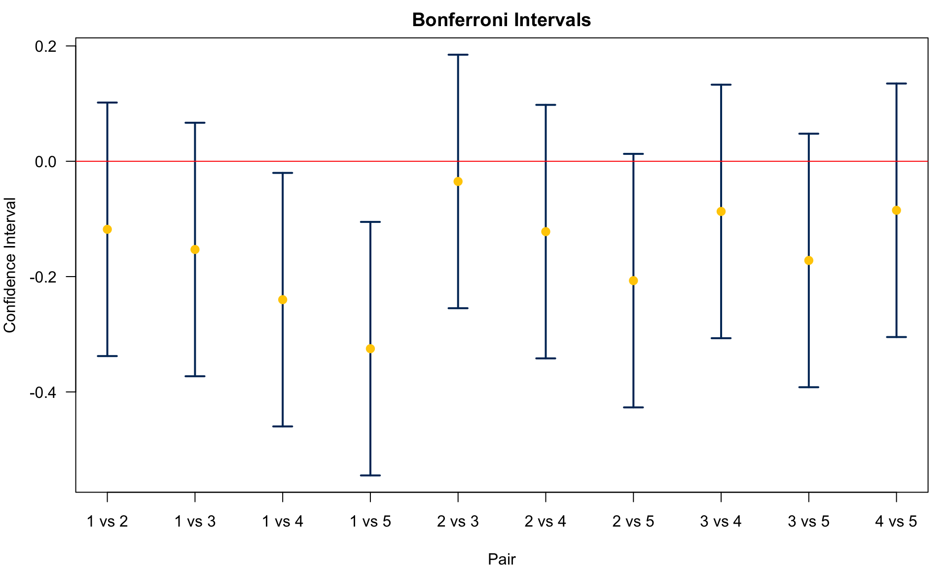
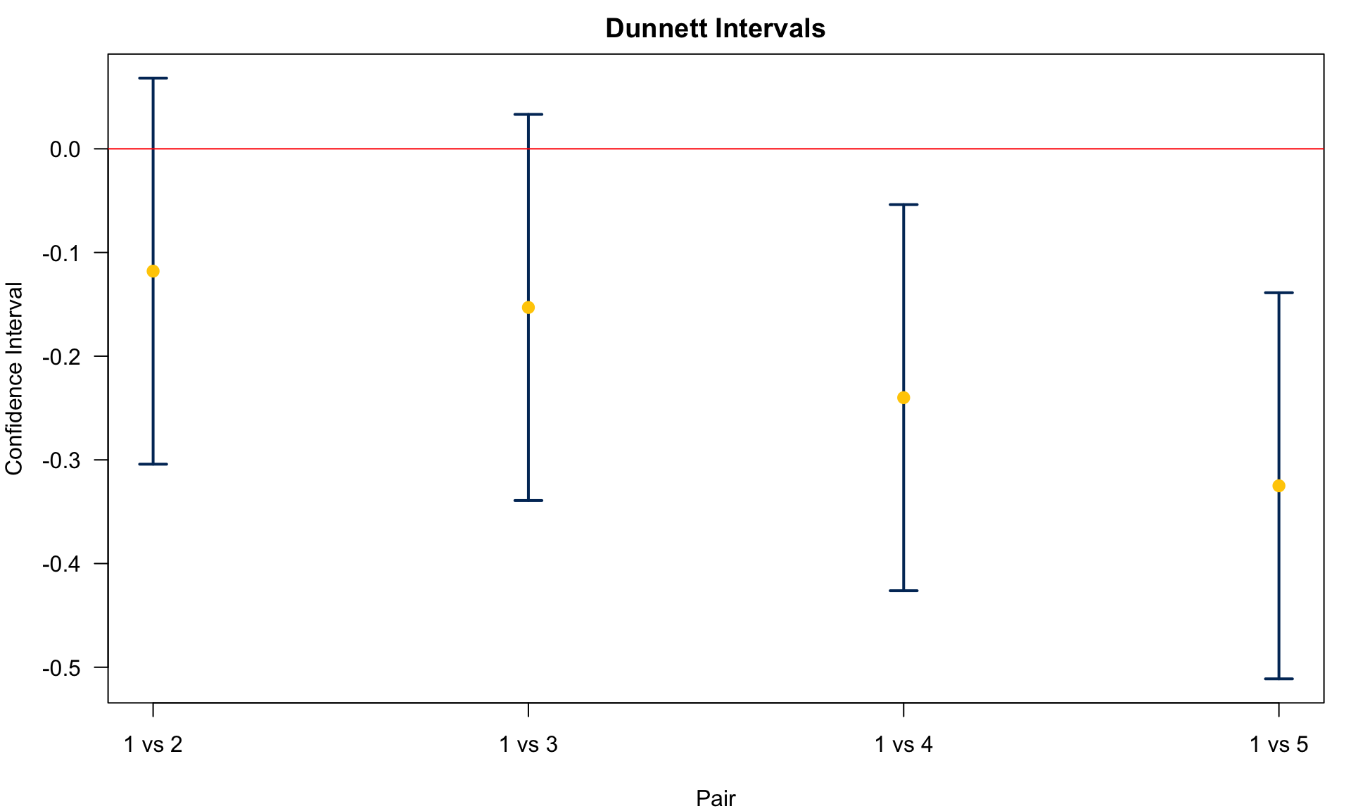
[10 rows x 8 columns]

For each pair, we can draw its confidence interval for $μ_{i} - μ_{j}$ . The CI formula is $({\overset{―}{y}}_{i} - {\overset{―}{y}}_{j}) \pm t_{\frac{α}{2 m}, d f_{W}} \sqrt{s_{W}^{2} (\frac{1}{n_{i}} + \frac{1}{n_{j}})}$ . The yellow dot represents ${\overset{―}{y}}_{i} - {\overset{―}{y}}_{j}$ . Centered at ${\overset{―}{y}}_{i} - {\overset{―}{y}}_{j}$ , we plus and minus the margin of error $t_{\frac{α}{2 m}, d f_{W}} \sqrt{s_{W}^{2} (\frac{1}{n_{i}} + \frac{1}{n_{j}})}$ to get the upper and lower bound of the CI. If the CI does not include zero, we conclude that $μ_{i}$ and $μ_{j}$ are not equal. Here again $μ_{1}$ and $μ_{4}$ are different. $μ_{1}$ and $μ_{5}$ are different too.

25.3 Fisher’s LSD (Least Significant Difference)

The second method introduced here is Fisher’s LSD, short for Least Significant Difference. We reject $H_{0}$ or say that pair $(μ_{i}, μ_{j})$ are significantly different if $| {\overset{―}{y}}_{i} - {\overset{―}{y}}_{j} | > t_{\frac{α}{2}, d f_{W}} \sqrt{s_{W}^{2} (\frac{1}{n_{i}} + \frac{1}{n_{j}})}$ Unlike the Bonferroni method, Fisher’s LSD does NOT correct for multiple comparisons or FWER. The diffrence between Bonferroni and Fisher’s LSD is that Bonferroni uses $α / m$ but Fisher’s LSD uses $α$ itself. The Fisher’s LSD test is basically a set of individual $t$ -tests. Two-sample pooled $t$ -tests compute the pooled variance from only the two groups being compared, while the Fisher’s LSD test computes the pooled variance from all the groups (which gains power). Also, the degrees fo freedom in the $t$ critical value is $d f_{W}$ , not $n_{i} + n_{j} - 2$ in the 2 sample pooled $t$ test.

Example of Multiple Comparison: Fisher’s LSD

 agent sample_mean sample_sd sample_size type
     1        1.17     0.120           6 None
     2        1.29     0.127           6 Bio1
     3        1.33     0.120           6 Bio2
     4        1.42     0.125           6 Chm1
     5        1.50     0.127           6 Chm2

The process of doing Fisher’s LSD is pretty similar to doing Bonferroni.

$\frac{α}{2} = 0.025$ , and $t_{0.025, 25} = 2.0595$
We conclude $μ_{i} - μ_{j} \neq 0$ if $| {\overset{―}{y}}_{i} - {\overset{―}{y}}_{j} | > 2.0595 \sqrt{0.0153 (\frac{1}{6} + \frac{1}{6})} = 0.1471$
Agent 1 v.s. 5: $| 1.500 - 1.175 | = 0.325 > 0.1471$
Agent 1 v.s. 4: $| 1.415 - 1.175 | = 0.240 > 0.1471$
Agent 1 v.s. 3: $| 1.328 - 1.175 | = 0.153 > 0.1471$
Agent 1 v.s. 2: $| 1.293 - 1.175 | = 0.118 < 0.1471$
Agent 2 v.s. 5: $| 1.500 - 1.293 | = 0.207 > 0.1471$
Agent 2 v.s. 4: $| 1.415 - 1.293 | = 0.112 < 0.1471$
Agent 2 v.s. 3: $| 1.328 - 1.293 | = 0.035 < 0.1471$
Agent 3, 4 and 5 are different from control. Agent 2 and 5 are different.

$| {\overset{―}{y}}_{i} - {\overset{―}{y}}_{j} | > t_{\frac{α}{2}, d f_{W}} \sqrt{s_{W}^{2} (\frac{1}{n_{i}} + \frac{1}{n_{j}})}$

R
Python

df

[1] 25

sw ^ 2

[1] 0.0153

(t_lsd <- qt(p = alpha/2, df = df, lower.tail = FALSE))

[1] 2.06

(E_lsd <- t_lsd * sw * sqrt(1/n + 1/n))

[1] 0.147

(y_bar_dist > E_lsd)

1 vs 2 1 vs 3 1 vs 4 1 vs 5 2 vs 3 2 vs 4 2 vs 5 3 vs 4 3 vs 5 4 vs 5 
 FALSE   TRUE   TRUE   TRUE  FALSE  FALSE   TRUE  FALSE   TRUE  FALSE

If we use pairwise.t.test(), pool.sd = TRUE because we do use the pooled variance $s_{W}^{2}$ that is pooled by all 5 samples. p.adjust.method = "none" because Fisher’s LSD does not adjust the Type I error rate. It still uses $α$ in every individual testing. The p-value result for every pair comparison shows that if $α = 0.05$ is the threshold or cutoff value, (1, 3), (1, 4), (1, 5), (2, 5), and (3, 5) pair comparisons reject their $H_{0}$ and conclude that there is a mean yield difference between their groups.

pairwise.t.test(data_weed$yield, data_weed$agent, pool.sd = TRUE, 
                p.adjust.method = "none") ## Fisher’s LSD


    Pairwise comparisons using t tests with pooled SD 

data:  data_weed$yield and data_weed$agent 

  1     2     3     4    
2 0.111 -     -     -    
3 0.042 0.628 -     -    
4 0.002 0.100 0.235 -    
5 1e-04 0.008 0.024 0.245

P value adjustment method: none

df

25.0

sw ** 2

0.015300990266666674

t_lsd = t.ppf(1 - alpha/2, df)
t_lsd

2.059538552753294

E_lsd = t_lsd * sw * np.sqrt(1/n + 1/n)
E_lsd

0.14708523139370552

y_bar_dist > E_lsd

array([False,  True,  True,  True, False, False,  True, False,  True,
       False])

The following should be replaced with LSD method which is still not found in any Python package. Need to update this.

pairwise_t_results = model_fit.t_test_pairwise(term_name='agent', method='bonferroni', alpha=0.05)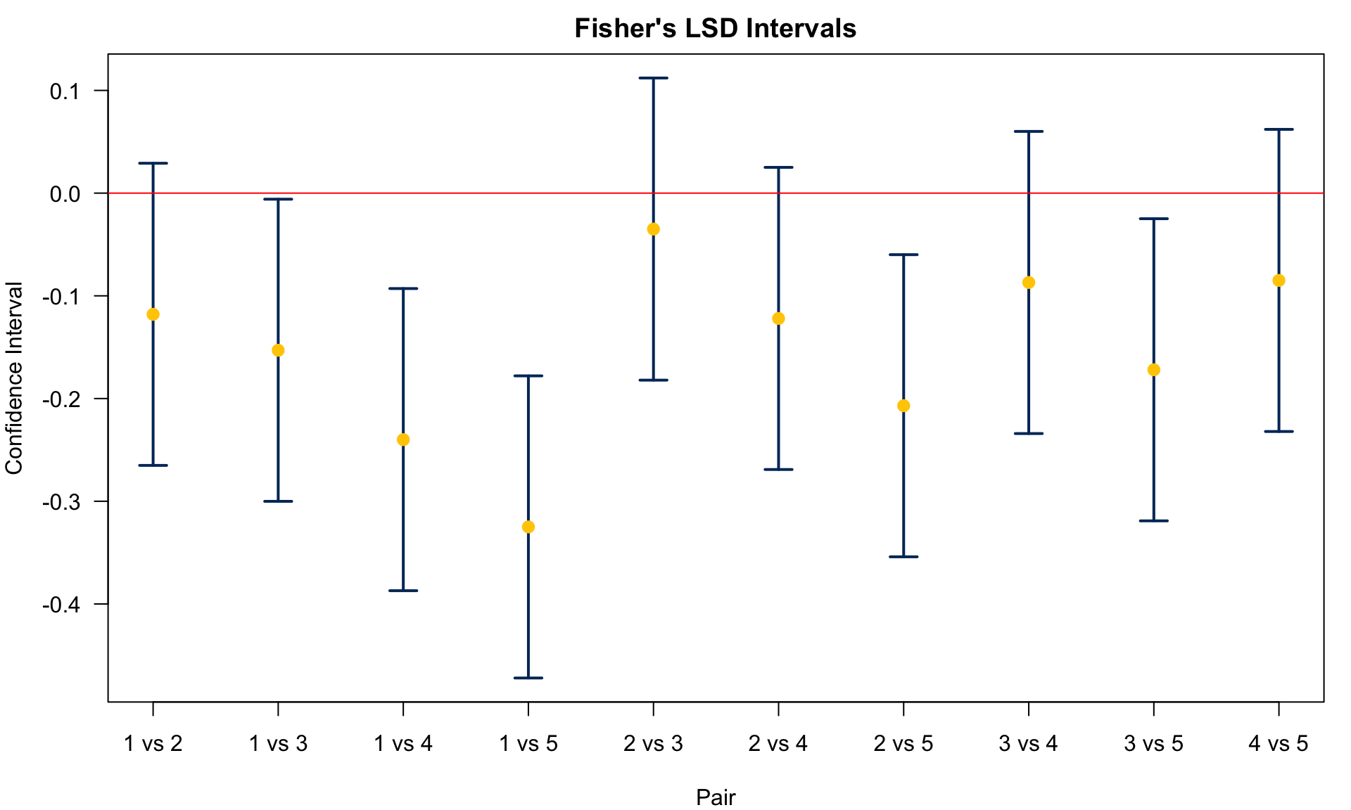
pairwise_t_results.result_frame

The Fisher’s LSD confidence interval for $μ_{i} - μ_{j}$ is $({\overset{―}{y}}_{i} - {\overset{―}{y}}_{j}) \pm t_{\frac{α}{2}, d f_{W}} \sqrt{s_{W}^{2} (\frac{1}{n_{i}} + \frac{1}{n_{j}})}$ . The CI for (1, 3), (1, 4), (1, 5), (2, 5), and (3, 5) do not include zero, leading to the same conclusion as the previous p-value method.

25.4 Tukey’s HSD (honestly significant difference)

The next method is the Tukey’s HSD method. We reject $H_{0}$ or say that pair $(μ_{i}, μ_{j})$ are significantly different if $| {\overset{―}{y}}_{i} - {\overset{―}{y}}_{j} | > \frac{q_{α} (t, d f_{W})}{\sqrt{2}} \sqrt{s_{W}^{2} (\frac{1}{n_{i}} + \frac{1}{n_{j}})}$

Here, the square root term or the standard error keeps the same as before, but we don’t use a $t$ critical value anymore. Instead, we use a different critical value $\frac{q_{α} (t, d f_{W})}{\sqrt{2}}$ , where $q_{α} (k, v)$ is the upper-tail critical value of the studentized range distribution for comparing $k$ different populations with degrees of freedom $v$ . Because we assume there are $t$ populations and df is $d f_{W}$ , I put them in the formula.

Studentized range distribution is similar to $t$ distribution when comparing 2 population means, but they are different things, and studentized range distribution actually controls FWER in some way but $t$ distribution does not. No need to worry about the details of this distribution. We just use it to apply the Tukey’s HSD method.

In R, we can use qtukey(p = alpha, nmeans = k, df = v, lower.tail = FALSE) to obtain $q_{α} (k, v)$ with specified $α$ , number of means to be compared $k$ , and the degrees of freedom $v$ . Notice that the $α$ here is the familywise error rate $α_{F}$ . We directly specify and control $α_{F}$ level, and the probability of falsely rejecting at least one pairwise tests is $α_{F}$ .

Example of Multiple Comparison: Tukey’s HSD

 agent sample_mean sample_sd sample_size type
     1        1.17     0.120           6 None
     2        1.29     0.127           6 Bio1
     3        1.33     0.120           6 Bio2
     4        1.42     0.125           6 Chm1
     5        1.50     0.127           6 Chm2

$k = 5$ , $d f_{W} = 25$ , $n = 6$ . Therefore, $q_{α} (k, v) = q_{0.05} (5, 25) = 4.153$ .
We conclude $μ_{i} - μ_{j} \neq 0$ if $| {\overset{―}{y}}_{i} - {\overset{―}{y}}_{j} | > 4.153 \sqrt{\frac{0.0153}{6}} = 0.2097$
Agent 1 v.s. 5: $| 1.500 - 1.175 | = 0.325 > 0.2097$
Agent 1 v.s. 4: $| 1.415 - 1.175 | = 0.240 > 0.2097$
Agent 1 v.s. 3: $| 1.328 - 1.175 | = 0.153 < 0.2097$
Agent 1 v.s. 2: $| 1.293 - 1.175 | = 0.118 < 0.2097$
Agent 2 v.s. 5: $| 1.500 - 1.293 | = 0.207 < 0.2097$
Agent 2 v.s. 4: $| 1.415 - 1.293 | = 0.112 < 0.2097$
Agent 2 v.s. 3: $| 1.328 - 1.293 | = 0.035 < 0.2097$
Agents 4 and 5 are different from control. No Significant difference between agents 3, 4, 5 and 2.

$| {\overset{―}{y}}_{i} - {\overset{―}{y}}_{j} | > q_{α} (k, d f_{W}) \sqrt{\frac{s_{W}^{2}}{n}}$

R
Python

df

[1] 25

sw^2

[1] 0.0153

(q_tukey <- qtukey(p = alpha, nmeans = 5, df = df, lower.tail = FALSE))

[1] 4.15

(E_tukey <- q_tukey * sw * sqrt(1 / n))

[1] 0.21

(y_bar_dist > E_tukey)

1 vs 2 1 vs 3 1 vs 4 1 vs 5 2 vs 3 2 vs 4 2 vs 5 3 vs 4 3 vs 5 4 vs 5 
 FALSE  FALSE   TRUE   TRUE  FALSE  FALSE  FALSE  FALSE  FALSE  FALSE

A faster way to conduct Tukey’s HSD test is to use R function TukeyHSD(). After doing ANOVA, we can save the result, say res_aov, then to implement Tukey method, just put the ANOVA result in the function TukeyHSD(). It will provide all information for each pair comparison.

res_aov <- aov(yield ~ agent, data = data_weed)
(tukey_test <- TukeyHSD(res_aov))

  Tukey multiple comparisons of means
    95% family-wise confidence level

Fit: aov(formula = yield ~ agent, data = data_weed)

$agent
     diff      lwr   upr p adj
2-1 0.118 -0.09172 0.328 0.480
3-1 0.153 -0.05672 0.363 0.234
4-1 0.240  0.03028 0.450 0.019
5-1 0.325  0.11526 0.535 0.001
3-2 0.035 -0.17474 0.245 0.988
4-2 0.122 -0.08774 0.332 0.447
5-2 0.207 -0.00276 0.417 0.054
4-3 0.087 -0.12274 0.297 0.741
5-3 0.172 -0.03776 0.382 0.146
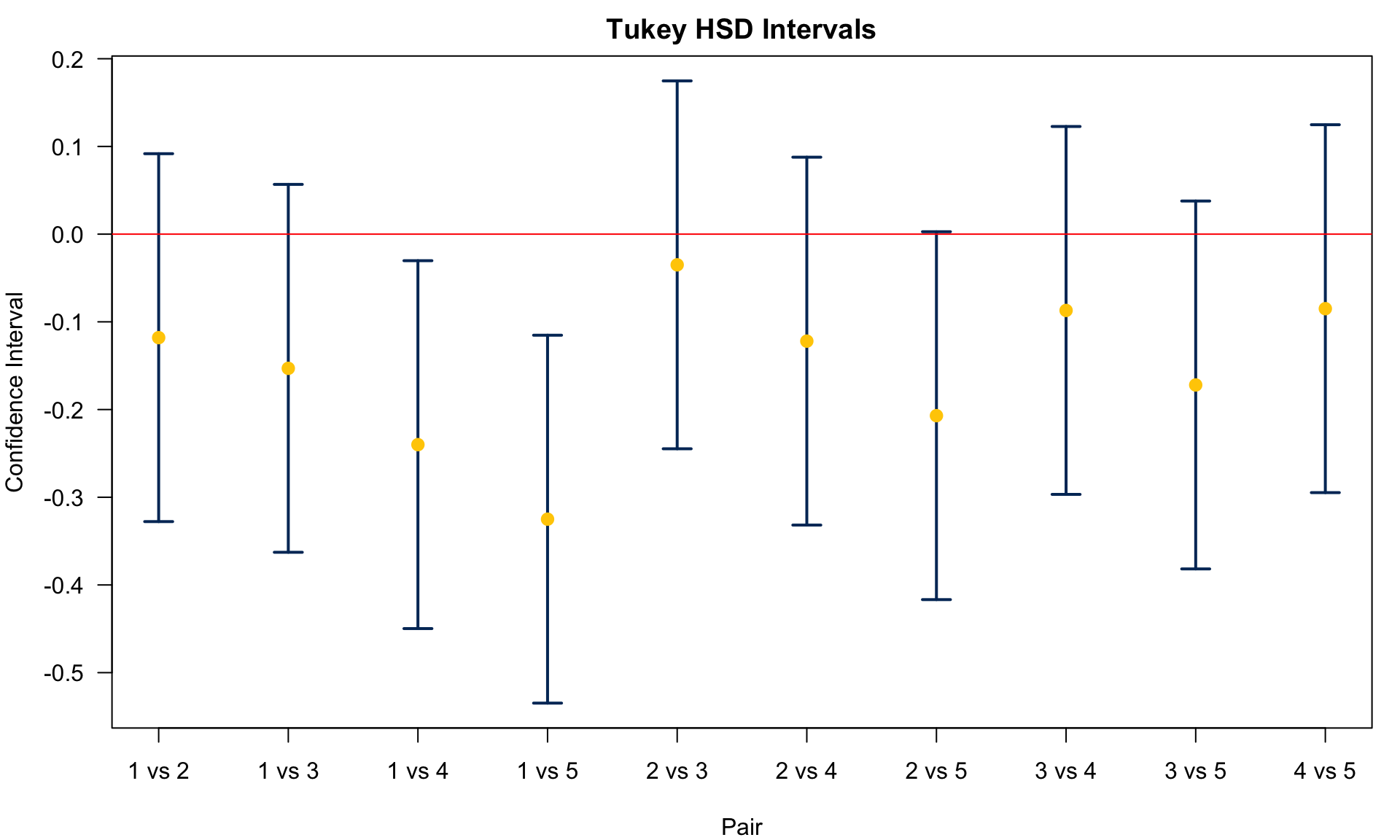
5-4 0.085 -0.12476 0.295 0.757

In the output, diff is ${\overset{―}{y}}_{i} - {\overset{―}{y}}_{j}$ where $i$ and $j$ are shown in the first column. lwr and upr are the lower bound and upper bound of the CI for $μ_{i} - μ_{j}$ , respectively. The adjusted p-values are shown in the p-adj column. With $α_{F} = 0.05$ , (4, 1) and (5, 1) are statistically discernible. Their corresponding lower bound is greater than zero, meaning that it’s CI for $μ_{i} - μ_{j}$ does not cover zero, so $μ_{i} - μ_{j}$ is statistically significantly different from zero.

The studentized range distribution in Python is implemented by the function studentized_range, again from scipy.stats.

df

25.0

sw**2

0.015300990266666674

from scipy.stats import studentized_range
q_tukey = studentized_range.ppf(q=1-alpha, k=5, df=df)
q_tukey

4.1533633299635335

E_tukey = q_tukey * sw * np.sqrt(1 / n)
E_tukey

0.2097413545569429

y_bar_dist > E_tukey

array([False, False,  True,  True, False, False, False, False, False,
       False])

A faster way to conduct Tukey’s HSD test is to use Python function pairwise_tukeyhsd() from statsmodels.stats.multicomp. It will provide all information for each pair comparison.

from statsmodels.stats.multicomp import pairwise_tukeyhsd
tukey = pairwise_tukeyhsd(endog=data_weed['yield_value'], 
                          groups=data_weed['agent'], alpha=0.05)
print(tukey)

Multiple Comparison of Means - Tukey HSD, FWER=0.05
===================================================
group1 group2 meandiff p-adj   lower  upper  reject
---------------------------------------------------
     1      2    0.118 0.4797 -0.0917 0.3278  False
     1      3    0.153 0.2342 -0.0567 0.3628  False
     1      4     0.24 0.0192  0.0303 0.4498   True
     1      5    0.325  0.001  0.1153 0.5347   True
     2      3    0.035 0.9876 -0.1747 0.2447  False
     2      4    0.122 0.4472 -0.0877 0.3317  False
     2      5    0.207 0.0543 -0.0028 0.4167  False
     3      4    0.087 0.7411 -0.1227 0.2967  False
     3      5    0.172 0.1461 -0.0378 0.3817  False
     4      5    0.085 0.7569 -0.1248 0.2947  False
---------------------------------------------------

In the output, meandiff is ${\overset{―}{y}}_{i} - {\overset{―}{y}}_{j}$ where $i$ and $j$ are shown in the first column. lower and upper are the lower bound and upper bound of the CI for $μ_{i} - μ_{j}$ , respectively. The last column represents p-values. With $α_{F} = 0.05$ , (4, 1) and (5, 1) are statistically discernible. Their corresponding lower bound is greater than zero, meaning that it’s CI for $μ_{i} - μ_{j}$ does not cover zero, so $μ_{i} - μ_{j}$ is statistically significantly different from zero.

25.5 Dunnett’s Method

The last but not least method introduced here is Dunnett’s method. We reject $H_{0}$ or say that pair $(μ_{i}, μ_{j})$ are significantly different if

$| {\overset{―}{y}}_{i} - {\overset{―}{y}}_{j} | > d_{α} (t - 1, d f_{W}) \sqrt{s_{W}^{2} (\frac{1}{n_{i}} + \frac{1}{n_{j}})}$

Well we still have the same standard error, the square root term, but we use another critical value $d_{α} (t - 1, d f_{W})$ . In general, for $d_{α} (k, d f)$ , the value of Dunnett’s test distribution, $k$ is the number of non-control groups or factors.

Note that this method is only used for comparing with a control or reference group. In our example, Agent 1 is the control group. So the parameter $k$ is $t - 1$ , where $t$ is the number of agents, which is 5. Again, the $α$ here is the familywise error rate $α_{F}$ . We directly specify and control $α_{F}$ level, and the probability of falsely rejecting at least one pairwise tests is $α_{F}$ .

Consider 2 treatment groups and one control group. If you only want to compare the 2 treatment groups with the control group, and do not want to compare the 2 treatment groups to each other, the Dunnett’s test is preferred.

Example of Multiple Comparison: Dunnett’s Method

$t - 1 = 4$ , $d f_{W} = 25$ , $n = 6$ . Therefore, $d_{α} (t - 1, d f_{W}) = d_{0.05} (4, 25) = 2.61$ .
We conclude $μ_{i} - μ_{j} \neq 0$ if $| {\overset{―}{y}}_{i} - {\overset{―}{y}}_{j} | > 2.61 \sqrt{\frac{2 (0.0153)}{6}} = 0.1862$
Agent 1 v.s. 5: $| 1.500 - 1.175 | = 0.325 > 0.1862$
Agent 1 v.s. 4: $| 1.415 - 1.175 | = 0.240 > 0.1862$
Agent 1 v.s. 3: $| 1.328 - 1.175 | = 0.153 < 0.1862$
Agent 1 v.s. 2: $| 1.293 - 1.175 | = 0.118 < 0.1862$
Only the chemical agents 4 and 5 are different from control. No biological agents are different from control.

$| {\overset{―}{y}}_{i} - {\overset{―}{y}}_{j} | > d_{α} (t - 1, d f_{W}) \sqrt{\frac{2 s_{W}^{2}}{n}}$

R
Python

There is no R built-in function that computes $d_{α}$ critical value. But we can install the package nCDunnett, and use the function qNCDun(). NC stands for Non-Central. The argument p is the probability to the left tail and keep in mind that the subscript $α$ in the critical value is the probability to the right tail. So we get to put $1 - α$ there. nu is the degrees of freedom. rho here we use 0.5, meaning that all sample sizes are equal. The sample size in each group is 6, and we need to specify it 4 times corresponding to the number of non-control groups. delta is the non-centrality parameter that needs to be specified 4 times too. Here we assume they are all zero, i.e., the test uses the central distribution.

library(nCDunnett)
(d_dun <- qNCDun(p = 1 - alpha, nu = df, 
                rho = c(0.5, 0.5, 0.5, 0.5), 
                delta = c(0, 0, 0, 0), two.sided = TRUE))

[1] 2.61

(E_dun <- d_dun * sw * sqrt(2 / n))

[1] 0.186

head(y_bar_dist > E_dun, 4)

1 vs 2 1 vs 3 1 vs 4 1 vs 5 
 FALSE  FALSE   TRUE   TRUE

DescTools.DunnettTest() performs Dunnett’s test that does multiple comparisons of means against a control group.

library(DescTools)


Attaching package: 'DescTools'

The following object is masked from 'package:car':

    Recode

The following object is masked from 'package:openintro':

    cards

DunnettTest(x=data_weed$yield, g=data_weed$agent)


  Dunnett's test for comparing several treatments with a control :  
    95% family-wise confidence level

$`1`
     diff  lwr.ci upr.ci    pval    
2-1 0.118 -0.0682  0.304 0.30737    
3-1 0.153 -0.0332  0.339 0.12931    
4-1 0.240  0.0538  0.426 0.00845 ** 
5-1 0.325  0.1387  0.511 0.00043 ***

---
Signif. codes:  0 '***' 0.001 '**' 0.01 '*' 0.05 '.' 0.1 ' ' 1

There is no functions in Python that calculates probabilities and quantiles of the Dunnett’s distribution.

scipy.stats.dunnett() performs Dunnett’s test that does multiple comparisons of means against a control group.

from scipy.stats import dunnett
dunnett_res = dunnett(data_weed[data_weed['agent'] == '2']['yield_value'], 
                      data_weed[data_weed['agent'] == '3']['yield_value'],
                      data_weed[data_weed['agent'] == '4']['yield_value'],
                      data_weed[data_weed['agent'] == '5']['yield_value'],
                      control=data_weed[data_weed['agent'] == '1']['yield_value'],
                      alternative='two-sided')
print(dunnett_res)

Dunnett's test (95.0% Confidence Interval)
Comparison               Statistic  p-value  Lower CI  Upper CI
 (Sample 0 - Control)      1.653     0.307    -0.068     0.304
 (Sample 1 - Control)      2.143     0.129    -0.033     0.339
 (Sample 2 - Control)      3.361     0.009     0.054     0.426
 (Sample 3 - Control)      4.551     0.000     0.139     0.511

The result shows (1, 4) and (1, 5) have different means. The figure below shows the CIs for $μ_{1} - μ_{j}, j = 2, 3, 4, 5$ .

Note

All comparisons illustrated are two-sided tests. One-sided tests can be applied too.

25.6 Comparison of Methods

To sum up, from the example, we had $μ_{i} - μ_{j} \neq 0$ if

Bonferroni: $| {\overset{―}{y}}_{i} - {\overset{―}{y}}_{j} | > 0.2198$
Fisher’s LSD: $| {\overset{―}{y}}_{i} - {\overset{―}{y}}_{j} | > 0.1471$
Tukey HSD: $| {\overset{―}{y}}_{i} - {\overset{―}{y}}_{j} | > 0.2097$
Dunnett: $| {\overset{―}{y}}_{i} - {\overset{―}{y}}_{j} | > 0.1862$
Fisher’s LSD does not control FWER, but all others do have FWER 0.05.
Bonferroni is the most conservative method and has the poorest discovery rate. You see its threshold value is the largest, making it the most difficult one to reject $H_{0}$ , and hence results in a lower power or lower discovery rate.
Discovery rate for the Tukey’s is better than Bonferroni, but not as good as Dunnett’s. However, Dunnett’s used only to compare with the control.
If the objective is to compare only with a control, then Dunnett’s is more powerful among three. Otherwise, Tukey’s is more powerful than Bonferroni.
Although Bonferroni is not very powerful, it does have advantage that it can be used in any situation (whether it is one factor or multi-factor analyses) whenever there are multiple hypotheses.
All methods here are based on the condition that the data are random samples from normal distributions with equal variances. There are nonparametric multiple comparison procedures out there, such as Kruskal–Wallis.
Here we focus on balanced data. When there are large differences in the number of samples, care should be taken when selecting multiple comparison procedures.

There is another method called Scheffe’s method. Unlike methods specifically for pairwise comparisons such as Tukey HSD, Scheffe’s method can generally investigate all possible contrasts of the means. In other words, it considers not only th pairwise comparisons but any possible combinations of the means, for example $c_{1} μ_{1} + c_{2} μ_{2} + \dots + c_{t} μ_{t}$ .

For pairwise comparisons, we reject $H_{0}$ or say that pair $(μ_{i}, μ_{j})$ are significantly different if

$| {\overset{―}{y}}_{i} - {\overset{―}{y}}_{j} | > \sqrt{(t - 1) F_{α, t - 1, N - t}} \sqrt{s_{W}^{2} (\frac{1}{n_{i}} + \frac{1}{n_{j}})}$ For pairwise comparisons, the Scheffé test has lower statistical power than other tests, even more conservative than Bonferroni method. To increase power, the Scheffé method needs larger sample size.