11  Continuous Probability Distributions

In this chapter, we discuss continuous probability distributions. We first learn the idea and properties of continuous distributions, then talk about probably the most important and commonly used distribution in probability and statistics, the normal distribution.

11.1 Introduction

Unlike a discrete random variable taking finite or countable values, a continuous random variable takes on any values from an interval of the real number line. For example, a continuous random variable \(X\) could take any value in the unit interval \([0, 1]\). Its possible values are uncountable.

Instead of probability functions, a continuous random variable \(X\) has the probability density function (pdf) denoted \(f(x)\) such that for any real value \(a < b\), \[P(a < X < b) = \int_{a}^b f(x) dx.\]

The probability that \(X\) is in some interval is computed from the integral of the density function with respect to \(x\). Keep in mind that the density function \(f(x)\) itself is not the probability that \(X = x\). The probability of continuous random variables is defined through the integral of \(f(x)\).

The cumulative distribution function (cdf) of \(X\) is defined as \[F(x) := P(X \le x) = \int_{-\infty}^x f(t)dt.\]

😎 Luckily, we don’t calculate integrals in this course. You just need to remember that for continuous random variables,

Important

• The pdf does not represent a probability.
• The integral of pdf represents a probability.
• The cdf itself by definition is a probability that is also from the integral of pdf.

Every probability density function must satisfy the two properties:

1. \(f(x) \ge 0\) for all \(x\) on the real line

2. \(\int_{-\infty}^{\infty} f(x) dx = 1\)

\(f(x)\) is a density value. For property 1, like density used in Physics, it cannot be negative. The density here represents how much likely the random variable \(X\) is around the value \(x\). When \(f(x) = 0\), it means that it is not possible to have \(X\) having value in the tiny neighborhood around \(x\). On the other hand, when \(f(x)\) is large, it is pretty likely to have \(X\) having values around \(x\). Because \(f(x)\) is the integrand, a larger value of \(f(x)\) in the interval \([a, b]\) will lead to a larger probability \(P(a < X < b)\).

The second property tells us that \(P(-\infty < X < \infty) = 1\). Remember that a random variable, whether it is discrete or continuous, must take a real value. Therefore the probability that \(X\) lives on the entire real line \((-\infty, \infty)\) is one.

In fact, any function satisfying the two properties can be served as a probability density function for some random variable.

---

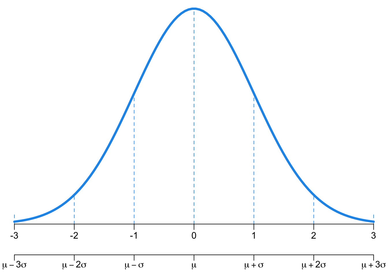
Density Curve

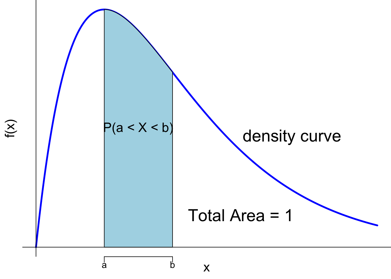
A probability density function generates a graph called a density curve that shows the likelihood of a random variable at all possible values. Figure 11.1 shows an example of density curve colored in blue. From Calculus 101, we have two important findings:

1. The integral of \(f(x)\) between \(a\) and \(b\) is actually the area under the density curve between \(a\) and \(b\). Therefore, the area under the density curve represents the probability \(P(a < X < b) = \int_{a}^b f(x) dx\), the density value \(f(x)\), or the height of the density curve does not.

2. The total area under any density curve is equal to 1: \(\int_{-\infty}^{\infty} f(x) dx = 1\).

Figure 11.1: Density curve for a random variable

Warning

Keep in mind that the area under the density curve represents probability, not the density value or the height of the density curve at some value of \(x\).

One question is for a continuous random variable \(X\), what is the probability that \(X\) equals any real number, or \(P(X = a)\) for any \(a \in \mathbf{R}\)? Since \(P(X = a) = P(a \le X \le a) = \int_{a}^a f(x) dx = 0\), we know that \(P(X = a) = 0\) for any real number \(a\). Graphically speaking, it means that there is no area under the density curve between \(a\) and \(a\).

Therefore, for a continuous random variable \(X\), \(P(a \le X\le b) = P(a < X < b)\) for any real value \(a\) and \(b\) because there is no probability mass on \(x = a\) and \(x = b\).

---

Commonly Used Continuous Distributions

There are tons of continuous distributions out there, and we won’t be able to discuss all of them. In this book, we will touch on normal (Gaussian), student’s t, chi-square, and F distributions. Some other popular distributions include uniform, exponential, gamma, beta, inverse gamma, Cauchy, etc. If you are interested in learning more distributions and their properties, please take a calculus-based probability theory course.

11.2 Normal (Gaussian) Distribution

We now discuss the most important distribution in probability and statistics, the normal distribution or Gaussian distribution.¹

The normal distribution, referred to as \(N(\mu, \sigma^2\)), has the probability density function given by \[\small f(x) = \frac{1}{\sqrt{2\pi}\sigma}e^{\frac{-(x-\mu)^2}{2\sigma^2}}, \quad -\infty < x < \infty,\] where the two parameters \(\mu\) and \(\sigma^2\) (\(\sigma\)) are the mean and variance (standard deviation) of the distribution respectively, i.e., \(E(X) = \mu\), and \(Var(X) = \sigma^2\) if \(X \sim N(\mu, \sigma^2)\). The normal variable \(X\) lives on the entire real line. The normal density value \(f(x)\) is not exactly equal to zero although it is tiny for extremely large \(x\) in absolute value. When \(\mu = 0\) and \(\sigma = 1\), \(N(0, 1)\) is called standard normal.

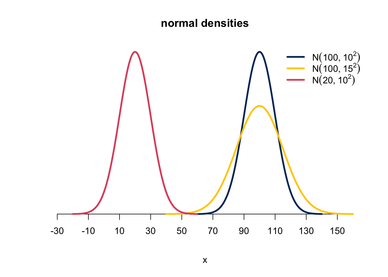
Figure 11.2 are examples of normal density curves and how they change with different means and standard deviations. The normal distribution is always bell-shaped and symmetric about the mean \(\mu\), regardless of the value of \(\mu\) and \(\sigma\). The parameter \(\mu\) is the location parameter that controls the “location” of the distribution. The navy \(N(100, 10^2)\) is 80 units right of the red \(N(20, 10^2)\). The parameter \(\sigma\) is the scale parameter that determines the variability or spreadness of the distribution. The navy \(N(100, 10^2)\) and the yellow \(N(100, 15^2)\) are at the same location, but \(N(100, 15^2)\) has more variation than \(N(100, 10^2)\). Since the total area under the density curve is always one, to account for large variation, the density curve of \(N(100, 15^2)\) has heavier tails and lower density values around the mean. Heavier tails means it is more probable to have extreme values like 130 or 70 that are away from the mean 100, comparing to \(N(100, 10^2)\) with smaller variation.

Figure 11.2: Normal density curves with varying means and standard deviations

11.3 Standardization and Z-Scores

Standardization is a transformation that allows us to convert any normal distribution \(N(\mu, \sigma^2)\) to \(N(0, 1)\), the standard normal distribution.

Why do we want to perform standardization? We want to put data on a standardized scale, because it helps us make comparisons more easily. Later we will see why. Let’s first see how we can do standardization.

If \(x\) is an observation from a distribution, not necessarily normal, with mean \(\mu\) and standard deviation \(\sigma\), the standardized value of \(x\) is called \(z\)-score: \[z = \frac{x - \mu}{\sigma}\]

The \(z\)-score tells us how many standard deviations \(x\) falls away from its mean and in which direction.

• Observations larger than the mean have positive \(z\)-scores.

• Observations smaller than the mean have negative \(z\)-scores.

• A \(z\)-score -1.2 means that \(x\) is 1.2 standard deviations to the left of or below the mean.

• A \(z\)-score 1.8 means that \(x\) is 1.8 standard deviations to the right of or above the mean.

If \(X \sim N(\mu, \sigma^2)\), then \(Z = \frac{X - \mu}{\sigma}\), the transformed random variable, follows the standard normal distribution \(Z \sim N(0, 1)\).

Note

Any transformation of a random variable is still a random variable but with a different probability distribution.

---

Graphical Illustration

What does the standardization really do? Well it first subtracts the original variable value \(x\) from the mean \(\mu\), then divided by its standard deviation \(\sigma\).

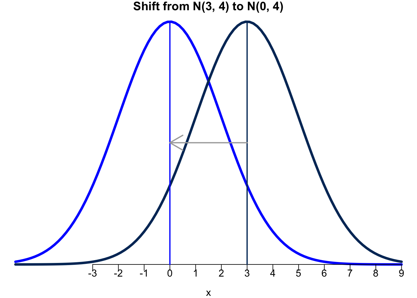
• First, \(X - \mu\) shifts the mean from \(\mu\) to 0. Figure 11.3 illustrates this. The original distribution is \(X \sim N(3, 4)\) (navy). Then the new variable \(Y = X-\mu\) is \(Y = X - 3\) that follows \(N(0, 4)\) distribution (blue). \(X - \mu\) means the distribution is shifted to the left 3 units, so that the new location or center becomes zero.

Figure 11.3: Standardization shifts mean from 3 to 0

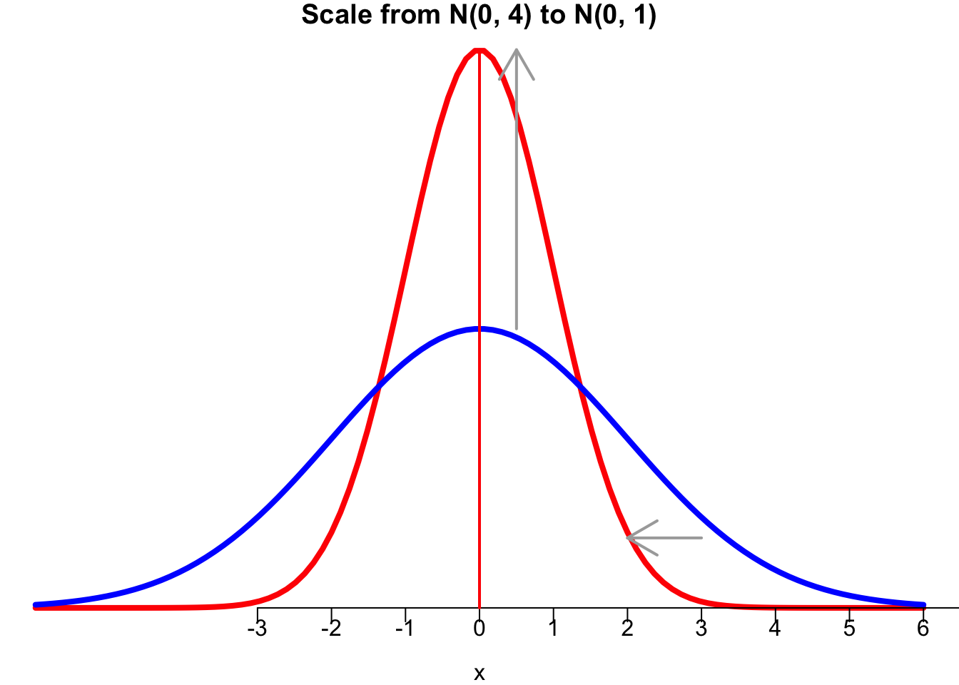
• Second, \(\frac{X - \mu}{\sigma}\) scales the variation from 4 to 1. \(Y = X-3 \sim N(0, 4).\) Because \(\sigma = 2\), \(Z = \frac{X - 3}{2} \sim N(0, 1)\). The idea is that one unit change in \(X\) is one unit change in \(Y\), but just 1/2 unit change in \(Z\). Through dividing by \(\sigma\), the variation measured in the new scale becomes smaller, and the new variance is one. For any normal variable with an arbitrary finite value of \(\mu\) and \(\sigma\), the variable after standardization will always follow \(N(0, 1)\) (red).

Figure 11.4: Standardization scales variance from 4 to 1

Note

If \(\sigma < 1\), then the variation measured in the new scale becomes larger, because the new variance is one.

A value of \(x\) that is 2 standard deviation below the mean, \(\mu\), corresponds to \(z = -2\). For any \(\mu\) and \(\sigma\), \(x\) and \(z\) have a one-to-one correspondence relationship: \(z = \frac{x -\mu}{\sigma} \iff x = \mu + z\sigma\). So if \(z = -2\), \(x = \mu - 2\sigma\). Figure 11.5 depicts how the values on the x-axis change when standardization is performed.

Figure 11.5: Standardized Normal Distribution

---

SAT and ACT Example (OS Example 4.2)

Standardization can help us compare the performance of students on the SAT and ACT, which both have nearly normal distributions. The table below lists the parameters for each distribution.

Measure	SAT	ACT
Mean	1100	21
SD	200	6

Suppose Anna scored a 1300 on her SAT and Tommy scored a 24 on his ACT. We want to determine whether Anna or Tommy performed better on their respective tests.

Standardization

Since SAT and ACT are measured on a different scale, we are not able to compare the two scores unless we measure them using the same scale. What we do is standardization. Both SAT and ACT are normally distributed but with different mean and variance. We first transform the two distributions into the standard normal distribution, then examining Anna and Tommys’ performance by checking the location of their score on the standard normal distribution.

The idea is that we first measure the two scores using the same scale and unit. The new transformed score in both cases is how many standard deviations the original score is away from its original mean. That is, both SAT and ACT are measured using the z-score. Then if A’s z-score is larger than B’ z-score, we know that A performs better than B because A has a relatively higher score than B.

The z-score of Anna and Tommy is \(z_{A} = \frac{x_{A} - \mu_{SAT}}{\sigma_{SAT}} = \frac{1300-1100}{200} = 1\); \(z_{T} = \frac{x_{T} - \mu_{ACT}}{\sigma_{ACT}} = \frac{24-21}{6} = 0.5\).

Figure 11.6: SAT and ACT distribution

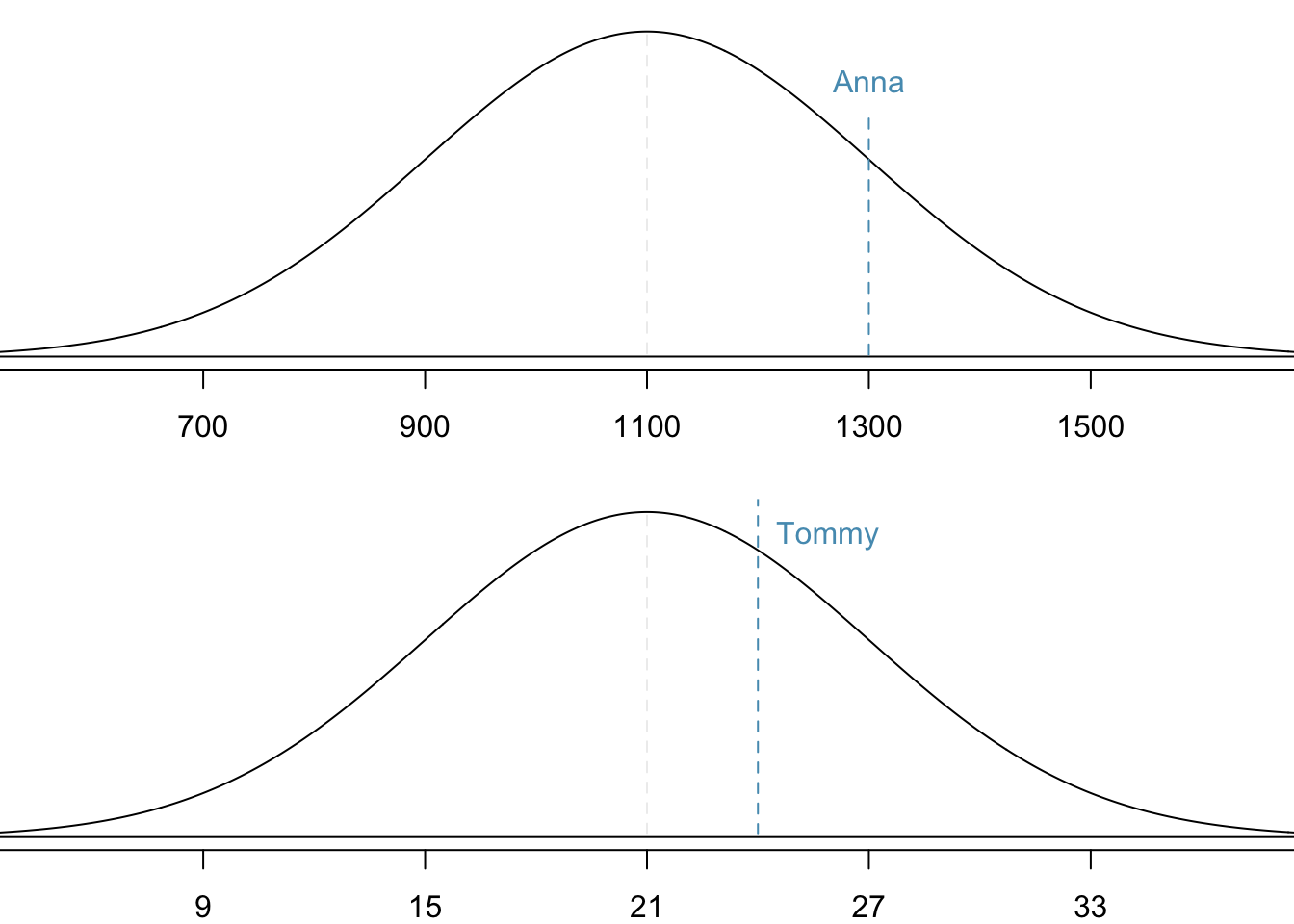
This standardization tells us that Anna scored 1 standard deviation above the mean and Tommy scored 0.5 standard deviations above the mean. From this information, we can conclude that Anna performed better on the SAT than Tommy performed on the ACT.

Figure 11.6 shows the SAT and ACT distributions. Note that the two distributions are depicted using the same density curve, as if they are measured on the same scale or standard normal distribution. Clearly we can see that Anna tends to do better with respect to everyone else than Tommy did.

11.4 Tail Areas and Normal Percentiles

Finding Tail Areas \(P(X < x)\)

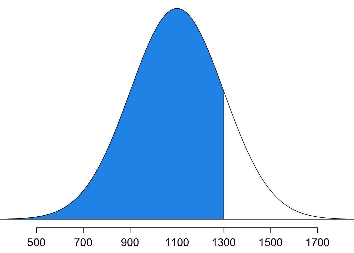
Finding tail areas allows us to determine the percentage of cases that are above or below a certain score. Going back to the SAT and ACT example, this can help us determine the fraction of students have an SAT score below Anna’s score of 1300. This is the same as determining what percentile Anna scored at, which is the percentage of cases that had lower scores than Anna. Therefore, we are looking for \(P(X < 1300 \mid \mu = 1100, \sigma = 200)\) or \(P(Z < 1 \mid \mu = 0, \sigma = 1)\) that corresponds to the blue area size shown in Figure 11.7. How? We can calculate this value using R.

Figure 11.7: Tail area for scores below 1300

R

With mean and sd representing the mean and standard deviation of a normal distribution, we use

• pnorm(q, mean, sd) to compute \(P(X \le q)\)

• pnorm(q, mean, sd, lower.tail = FALSE) to compute \(P(X > q)\)

pnorm(1, mean = 0, sd = 1)

[1] 0.8413447

pnorm(1300, mean = 1100, sd = 200)

[1] 0.8413447

Python

With loc and scale representing the mean and standard deviation of a normal distribution, we use

• norm.cdf(x, loc, scale) to compute \(P(X \le x)\)

• norm.sf(x, loc, scale) to compute \(P(X > x)\)

from scipy.stats import norm, binom

norm.cdf(x=1, loc=0, scale=1)

0.8413447460685429

norm.cdf(1300, loc=1100, scale=200)

0.8413447460685429

Notice that the z-score 1 in standard normal is equivalent to 1300 in \(N(1100, 200^2)\). The shaded area represents the 84.1% of SAT test takers who had z-score below 1.

Second ACT and SAT Example

Shannon is an SAT taker, and nothing else is known about her SAT aptitude. With SAT score following \(N(1100, 200^2)\), what is the probability Shannon SAT score is at least 1190?

Let’s get the probability step by step. The first step is to figure out the probability we want to compute from the description of the question.

• Step 1: State the problem
  • We want to compute \(P(X \ge 1190)\).

If you are an expert like me, you may already know how to get the probability using R once you know what you want to compute. But if you are a beginner, I strongly recommend you drawing a normal picture, and figure out which area is your goal.

• Step 2: Draw a picture

Figure 11.8: Tail area for scores greater than 1190

Figure 11.9: Method to determine right tail areas

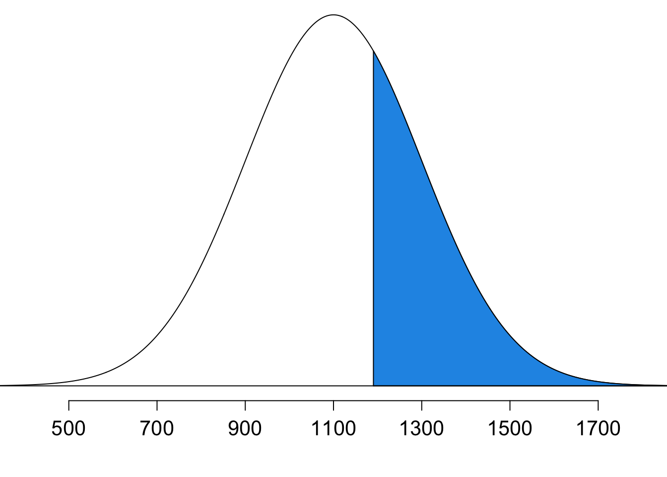
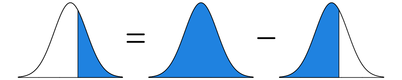
Note that Figure 11.9 reflects the fact that \(P(X \ge 1190) = 1 - P(X < 1190).\) The area on the right is equal to the whole area which is one minus the area on the left.

The next step, which is not necessary, is to find the z-score. Using z-scores help us write shorter R code to compute the wanted probability.

• Step 3: Find \(z\)-score

\(z = \frac{1190 - 1100}{200} = 0.45\) and we want to compute \(\begin{align*} P(X > 1190) &= P\left( \frac{X - \mu}{\sigma} > \frac{1190 - 1000}{200} \right) \\&= P(Z > 0.45) = 1 - P(Z \le 0.45) \end{align*}\)

At this point, we obtain the target probability once we get \(P(Z \le 0.45)\). The last step is to use pnorm() function to get it done.

R

• Step 4: Find the area using pnorm()

1 - pnorm(0.45)

[1] 0.3263552

Note

When we use R pnorm() to compute normal probabilities, standardization is not a must. However, if we don’t use z-scores, we must specify the mean and SD of the original distribution of \(X\), like pnorm(x, mean = mu, sd = sigma). Otherwise, R does not know which normal distribution we are considering. For example,

1 - pnorm(1190, mean = 1100, sd = 200)

[1] 0.3263552

By default, pnorm() uses the standard normal distribution assuming mean = 0 and sd = 1. So if we use z-scores to compute probabilities, we don’t need to specify the value of mean and standard deviation, and our code is shorter:

1 - pnorm(0.45)

[1] 0.3263552

Note

Any probability can be computed using the “less than” form (lower or left tail). In the previous example, we use \(P(X \ge 1190) = 1 - P(X < 1190)\) expression, and we find \(P(X < 1190)\) that has the “less than” form.

This step is not necessary too, and we can directly compute \(P(X \ge 1190)\) using pnorm(). However, if the calculation involves the “greater than” form, or we focus on upper or right tail part of the distribution, we need to add lower.tail = FALSE in pnorm(). For example,

pnorm(1190, mean = 1100, sd = 200, lower.tail = FALSE)

[1] 0.3263552

By default, lower.tail = TRUE, and pnorm(q, ...) finds a probability \(P(X < q)\), the lower tail part of the distribution.

Python

• Step 4: Find the area using norm.cdf()

1 - norm.cdf(0.45)

0.32635522028791997

Note

When we use Python norm.cdf() to compute normal probabilities, standardization is not a must. However, if we don’t use z-scores, we must specify the mean and SD of the original distribution of \(X\), like norm.cdf(x, loc= mu, scale=sigma). Otherwise, Python does not know which normal distribution we are considering. For example,

1 - norm.cdf(1190, loc=1100, scale=200)

0.32635522028791997

By default, norm.cdf() uses the standard normal distribution assuming loc=0 and scale=1. So if we use z-scores to compute probabilities, we don’t need to specify the value of mean and standard deviation, and our code is shorter:

1 - norm.cdf(0.45)

0.32635522028791997

Note

Any probability can be computed using the “less than” form (lower or left tail). In the previous example, we use \(P(X \ge 1190) = 1 - P(X < 1190)\) expression, and we find \(P(X < 1190)\) that has the “less than” form.

This step is not necessary too, and we can directly compute \(P(X \ge 1190)\) using norm.sf(). For example,

norm.sf(1190, loc=1100, scale=200)

0.32635522028791997

---

Normal Percentiles in R

Quite often we want to know what score we need to get in order to be in the top 10% of the test takers, or the minimal score we should get to be not at the bottom 20%. To answer such questions, we need to find the percentile or quantile of the underlying distribution.

To get the \(100p\)-th percentile (or the \(p\) quantile denoted as \(q\) ) of a normal distribution, given probability \(p\), we use

R

• qnorm(p, mean, sd) to get a value of \(X\), \(q\), such that \(P(X \le q) = p\)

• qnorm(p, mean, sd, lower.tail = FALSE) to get \(q\) such that \(P(X \ge q) = p\)

Python

• norm.ppf(p, loc, scale) to get a value of \(X\), \(x\), such that \(P(X \le x) = p\)

• norm.isf(p, loc, scale) to get \(x\) such that \(P(X \ge x) = p\). isf is short for inverse survival function.

SAT and ACT Example

Back to our SAT example. What is the 95th percentile for SAT scores?

Keep in mind that a percentile or quantile is a value of random variable \(x\), not a probability. When we find the quantile, its associated probability is given because the probability is the required information to obtain the quantile.

The first step again is to figure out what we want. If we want to find the 95th percentile, it means that we want to find the variable value \(q\) so that \(P(X < q) = 0.95\). In other words, we want to find an \(x\) value of the normal distribution, which is greater than 95% of all other cases.

• Step 1: State the problem
  • We want to find \(q\) s.t \(P(X < q) = 0.95\).

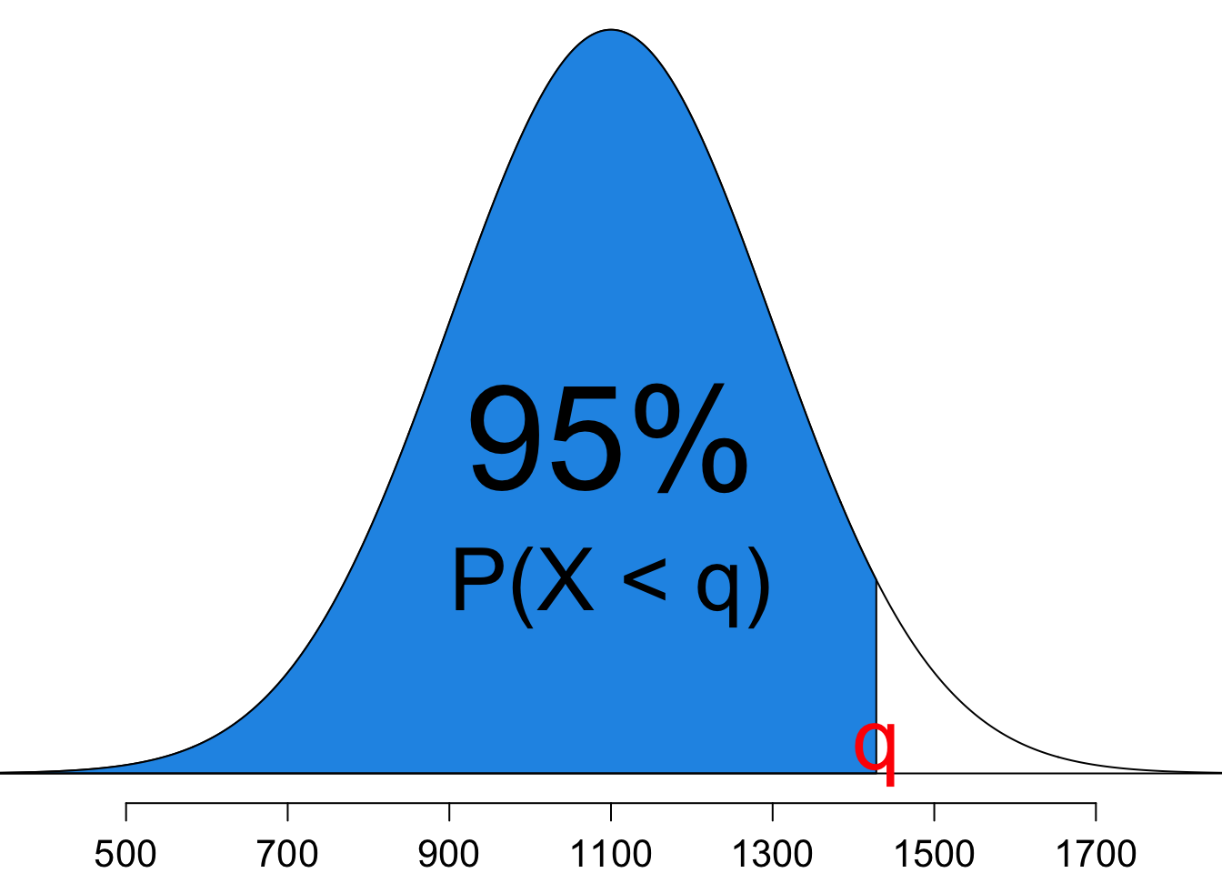
The whole idea is shown graphically in Figure 11.10. We already know the percentage 95%. All we need to do is to find the value \(q\) so that the area left to it is 95%.

• Step 2: Draw a picture

Figure 11.10: Picture for the 95th percentile of SAT scores

Like we do in finding probabilities, we can first do the standardization for finding quantiles although it is not necessary. So we use qnorm() to find the z-score \(z^*\), or the value of a standard normal variable that is the 95th percentile, i.e., \(P(Z < z^*) = 0.95\).

R

• Step 3: Find \(z\)-score s.t. \(P(Z < z^*) = 0.95\) using qnorm():

(z_95 <- qnorm(0.95))

[1] 1.644854

Now, since we are interested in the 95th percentile of SAT, not the z-score, we need to transform the 95th percentile of \(N(0, 1)\) back to the 95th percentile of \(N(1100, 200^2)\), the original SAT distribution.

• Step 4: Find the \(x\) of the original scale
  • \(z_{0.95} = \frac{x-\mu}{\sigma}\). So \(x = \mu + z_{0.95}\sigma = 1100+(1.645)\times200 = 1429\).

(x_95 <- 1100 + z_95 * 200)

[1] 1428.971

Therefore, the 95th percentile for SAT scores is 1429.

Note that we can directly find the 95th percentile of SAT without standardization. We just need to remember to stay in the original SAT distribution by explicitly specifying mean = 1100 and sd = 200 in the qnorm() function, as we do for pnorm().

qnorm(p = 0.95, mean = 1100, sd = 200)

[1] 1428.971

Python

• Step 3: Find \(z\)-score s.t. \(P(Z < z^*) = 0.95\) using norm.ppf():

z_95 = norm.ppf(0.95)
z_95

1.6448536269514722

Now, since we are interested in the 95th percentile of SAT, not the z-score, we need to transform the 95th percentile of \(N(0, 1)\) back to the 95th percentile of \(N(1100, 200^2)\), the original SAT distribution.

• Step 4: Find the \(x\) of the original scale
  • \(z_{0.95} = \frac{x-\mu}{\sigma}\). So \(x = \mu + z_{0.95}\sigma = 1100+(1.645)\times200 = 1429\).

x_95 = 1100 + z_95 * 200
x_95

1428.9707253902943

Therefore, the 95th percentile for SAT scores is 1429.

Note that we can directly find the 95th percentile of SAT without standardization. We just need to remember to stay in the original SAT distribution by explicitly specifying loc=1100 and scale=200 in the norm.ppf() function, as we do for norm.cdf().

norm.ppf(0.95, loc=1100, scale=200)

1428.9707253902943

11.5 Finding Probabilties

R

👉 To find a probability, if you are a beginner, it is always good to draw and label the normal curve and shade the area of interest. Below is a summary of how we can use pnorm() to compute various kinds of probabilities.

• 👉 Less than
  • \(\small P(X < x) = P(Z < z)\)
  • pnorm(z)
  • pnorm(x, mean = mu, sd = sigma)
• 👉 Greater than
  • \(\small P(X > x) = P(Z > z) = 1 - P(Z \le z)\)
  • 1 - pnorm(z)
  • 1 - pnorm(x, mean = mu, sd = sigma)
  • pnorm(x, mean = mu, sd = sigma, lower.tail = FALSE)

• 👉 Between two numbers

  • \(\small P(a < X < b) = P(z_a < Z < z_b) = P(Z < z_b) - P(Z < z_a)\)
  • pnorm(z_b) - pnorm(z_a)
  • pnorm(b, mean = mu, sd = sigma) - pnorm(a, mean = mu, sd = sigma)

• 👉 Outside of two numbers \((a < b)\) \[\small \begin{align} P(X < a \text{ or } X > b) &= P(Z < z_a \text{ or } Z > z_b) \\ &= P(Z < z_a) + P(Z > z_b) \\ &= P(Z < z_a) + 1 - P(Z < z_b) \end{align}\]

  • pnorm(z_a) + pnorm(z_b, lower.tail = FALSE)
  • pnorm(z_a) + 1 - pnorm(z_b)
  • pnorm(a, mean = mu, sd = sigma) + pnorm(b, mean = mu, sd = sigma, lower.tail = FALSE)
  • pnorm(a, mean = mu, sd = sigma) + 1 - pnorm(b, mean = mu, sd = sigma)

Python

👉 To find a probability, if you are a beginner, it is always good to draw and label the normal curve and shade the area of interest. Below is a summary of how we can use norm.cdf() and norm.sf() to compute various kinds of probabilities.

• 👉 Less than
  • \(\small P(X < x) = P(Z < z)\)
  • norm.cdf(z)
  • norm.cdf(x, loc=mu, scale=sigma)
• 👉 Greater than
  • \(\small P(X > x) = P(Z > z) = 1 - P(Z \le z)\)
  • 1 - norm.cdf(z)
  • 1 - norm.cdf(x, loc=mu, scale=sigma)
  • norm.sf(x, loc=mu, scale=sigma)

• 👉 Between two numbers

  • \(\small P(a < X < b) = P(z_a < Z < z_b) = P(Z < z_b) - P(Z < z_a)\)
  • norm.cdf(z_b) - pnorm.cdf(z_a)
  • norm.cdf(b, loc=mu, scale=sigma) - norm.cdf(a, loc=mu, scale=sigma)

• 👉 Outside of two numbers \((a < b)\) \[\small \begin{align} P(X < a \text{ or } X > b) &= P(Z < z_a \text{ or } Z > z_b) \\ &= P(Z < z_a) + P(Z > z_b) \\ &= P(Z < z_a) + 1 - P(Z < z_b) \end{align}\]

  • norm.cdf(z_a) + norm.sf(z_b)
  • norm.cdf(z_a) + 1 - norm.cdf(z_b)
  • norm.cdf(a, loc=mu, scale=sigma) + norm.sf(b, loc=mu, scale=sigma)
  • norm.cdf(a, loc=mu, scale=sigma) + 1 - norm.cdf(b, loc=mu, scale=sigma)

11.6 Checking Normality

11.6.1 Normal quantile plot

If we use a statistical method with its assumption being violated, the analysis results and conclusion made by the method will be worthless. Many statistical methods assume variables are normally distributed. Therefore, testing the appropriateness of the normal assumption is a key step.

We can check this normality assumption using a so-called normal quantile plot (normal probability plot) or a Quantile-Quantile plot (QQ plot).

The construction of the QQ plot is technical, and we don’t need to dig into that at this moment. The bottom line is if the data are (nearly) normally distributed, the points on the QQ plot will lie close to a straight line.

If the data are right-skewed, the points on the QQ plot will be convex-shaped. If the data are left-skewed, the points on the QQ plot will be concave-shaped.

R

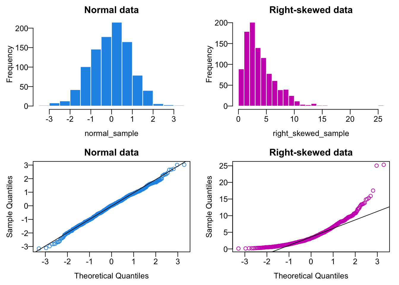
To generate a QQ-plot for checking normality in R, we can use qqnorm() and qqline(), where the first argument in the functions is the sample data we would like to check. Figure 11.11 shows QQ plots at the bottom for normal and right-skewed data samples. Since the data normal_sample actually come from a normal distribution, its histogram looks like normal, and its QQ plot look like a perfect straight line. On the other hand, on the right hand side we have a right skewed data set right_skewed_sample. Clearly, its QQ plot is a upward curve, and definitely not linear, indicating that the sample data are not normally distributed.

qqnorm(normal_sample, main = "Normal data", col = 4)
qqline(normal_sample)
qqnorm(right_skewed_sample, main = "Right-skewed data", col = 6)
qqline(right_skewed_sample)

Figure 11.11: QQ plots for normal and right-skewed data samples

Python

To generate a QQ-plot for checking normality in R, we can use stats.probplot(), where the first argument in the functions is the sample data we would like to check. Figure 11.12 shows QQ plots at the bottom for normal and right-skewed data samples. Since the data normal_sample actually come from a normal distribution, its histogram looks like normal, and its QQ plot look like a perfect straight line. On the other hand, on the right hand side we have a right skewed data set right_skewed_sample. Clearly, its QQ plot is a upward curve, and definitely not linear, indicating that the sample data are not normally distributed.

import numpy as np
import scipy.stats as stats
import matplotlib.pyplot as plt

# First plot: Histogram of normal data
nor_hist = axs[0, 0].hist(normal_sample, bins=20, color='blue', edgecolor='white')
axs[0, 0].set_title("Normal data")
axs[0, 0].set_xlabel("Value")
axs[0, 0].set_ylabel("Frequency")

# Second plot: QQ plot for normal data
nor_qq = stats.probplot(normal_sample, dist="norm", plot=axs[1, 0])
axs[1, 0].set_title("Normal data (QQ Plot)")

# Third plot: Histogram of right-skewed data
skew_hist = axs[0, 1].hist(right_skewed_sample, bins=20, color='magenta', edgecolor='white');
axs[0, 1].set_title("Right-skewed data")
axs[0, 1].set_xlabel("Value")
axs[0, 1].set_ylabel("Frequency")

# Fourth plot: QQ plot for right-skewed data
skew_qq = stats.probplot(right_skewed_sample, dist="norm", plot=axs[1, 1])
axs[1, 1].get_lines()[0].set_markerfacecolor('magenta')
axs[1, 1].set_title("Right-skewed data (QQ Plot)")

# Display the plots
plt.show()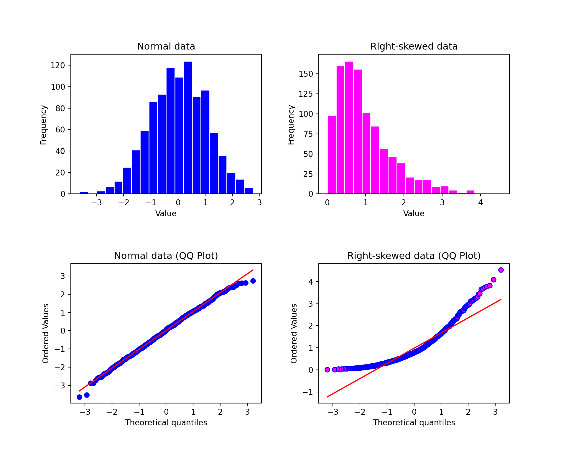

Figure 11.12: QQ plots for normal and right-skewed data samples

Note

The code involves doing subplots in one single figure, and it makes the code a bit complex and long. No need to worry that much.

11.6.2 Normality test

If visualization is not enough for you to tell whether the data are far from normally distributed, we can use some formal procedures to make such conclusion. Since the methods are about hypothesis testing which will be first introduced in Chapter 16, we will take about normality test in later chapters after we learn hypothesis testing.

11.7 Normal Approximation to Binomial Distribution*

In Chapter 10, we learn that a binomial distribution can be approximated by a Poisson distribution. In this section we learn that a binomial distribution can also be approximated by a normal distribution. How good the approximation is again depends on the size of \(n\) and \(\pi\). Centuries ago, with no computing technology, calculating binomial probabilities is a pain in the neck, especially when \(n\) is large. This motivates mathematicians to find another way to calculate the probabilities, or at least approximate them well. Not only binomial distributions, many other distributions are related to the normal distribution. This will be discussed in a probability theory course.

To determine a normal distribution, we need parameters \(\mu\) and \(\sigma\). We know that if \(X \sim Binomial(n, \pi)\), then the mean and standard deviation of \(X\) are \[ \begin{align} \mu &= n\pi,\\ \sigma &= \sqrt{n\pi(1-\pi)}. \end{align}\]

When \(n\) is large, we can approximate \(X\) with a normal distribution \(N\left(\mu = n\pi, \sigma^2 = n\pi(1-\pi)\right)\). When this normal approximation does a pretty good job? Usually, the normal approximation performs well when \(n\) is so large that \(n\pi \ge 5\) and \(n(1-\pi) \ge 5\). As you can see, when \(\pi\) is near 0 or 1, \(n\) needs to be much larger to satisfy the two conditions. The intuition is that normal distributions are symmetric, but binomial distributions are generally asymmetric. The more \(\pi\) is close to 0 or 1, the more asymmetric the binomial distribution is, unless \(n\) gets larger.

Can you see any potential issue of using normal to approximate binomial? In fact, we are using a continuous normal distribution to approximate a discrete binomial distribution. In order to have a good approximation, especially when \(n\) is not that large, we need something called continuity correction.

Continuity correction is made to transform discrete binomial values \(0, 1, 2, \dots, n\) to a continuous interval from 0 to \(n\) by adding and subtracting 0.5 from the whole number \(0, 1, 2, \dots, n\).

Figure 11.13

By doing so, \(P_{Binomial}(X = k) \approx\) integral of normal from \(k-0.5\) to \(k+0.5\). The idea is that in normal distribution, we treat any value between 0.5 and 1.5 as an integer 1 of the value of the discrete binomial distribution. The followings are some examples of continuity correction.

• \(P_{Binomial}(X \ge 1) \approx P_{Normal}(X > 0.5)\).

• \(P_{Binomial}(X > 1) \approx P_{Normal}(X > 1.5)\)

• \(P_{Binomial}(X \le 4) \approx P_{Normal}(X < 4.5)\)

• \(P_{Binomial}(X < 4) \approx P_{Normal}(X < 3.5)\)

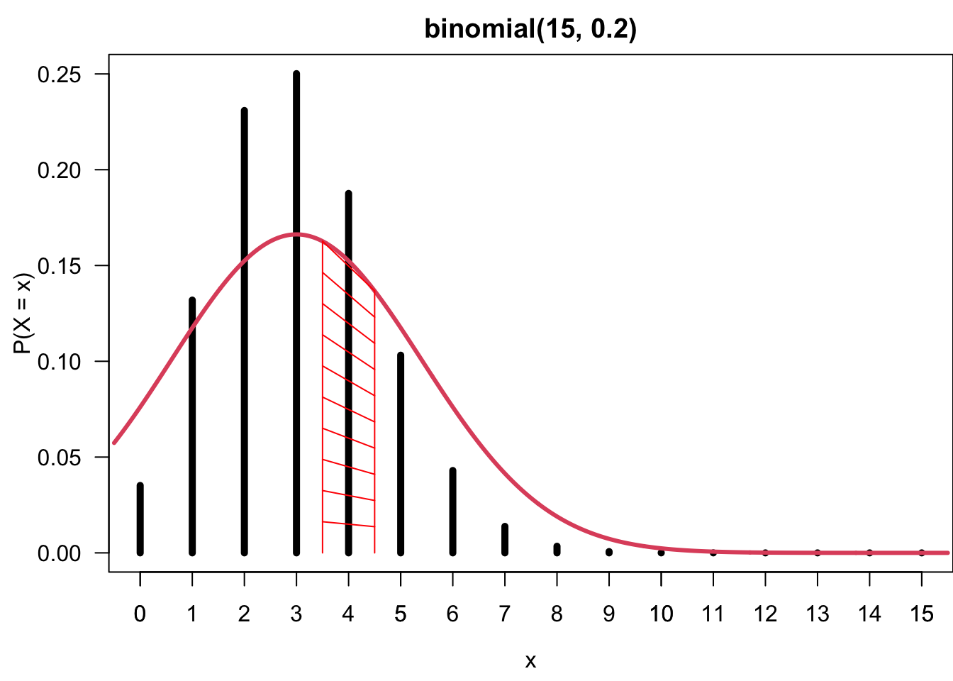
• \(P_{Binomial}(X = 4) \approx P_{Normal}(3.5 < X < 4.5)\)

Figure 11.13 illustrate that \(P_{Binomial}(X = 4) \approx P_{Normal}(3.5 < X < 4.5)\). The height of the black bar at \(x = 4\) is 0.187 showing \(P_{Binomial}(X = 4)\) with \(X \sim binomial(15, 0.2)\). This can be approximated by the integral of the normal density curve between 3.5 and 4.5, the red shaded area, which is \(P_{Normal}(3.5 < X < 4.5)\) where \(X \sim N(15(0.2), 15(0.2)(0.8))\).

---

Example of Normal Approximation (4.26 of OTT)

A large drug company has 100 potential new prescription drugs under clinical test. About 20% of all drugs that reach this stage are eventually licensed for sale. What is the probability that at least 15 of the 100 drugs are eventually licensed?

R

n <- 100  # number of trials
p <- 0.2  # probability of being licensed for sale

## 1. Exact Binomial Probability P(X >= 15) = 1 - P(X < 14)
1 - pbinom(q = 14, size = n, prob = p)

[1] 0.9195563

## 2. Normal approximation with Continuity Correction 
## P(X >= 14.5) = 1 - P(X < 14.5)
1 - pnorm(q = 14.5, mean = n * p, sd = sqrt(n * p * (1 - p)))

[1] 0.9154343

## 3. Normal approximation with NO Continuity Correction 
## P(X >= 15) = 1 - P(X < 15)
1 - pnorm(q = 15, mean = n * p, sd = sqrt(n * p * (1 - p)))

[1] 0.8943502

Python

n = 100  # number of trials
p = 0.2  # probability of success

from scipy.stats import norm, binom

# 1. Exact Binomial Probability P(X >= 15) = 1 - P(X < 15)
1 - binom.cdf(14, n, p)

0.9195562788619489

# 2. Normal approximation with continuity correction
1 - norm.cdf(14.5, loc=n * p, scale=np.sqrt(n * p * (1 - p)))

0.9154342776486644

# 3. Normal approximation without continuity correction
1 - norm.cdf(15, loc=n * p, scale=np.sqrt(n * p * (1 - p)))

0.8943502263331446

11.8 Exercises

1. What percentage of data that follow a standard normal distribution \(N(\mu=0, \sigma=1)\) is found in each region? Drawing a normal graph may help.
   1. \(Z < -1.75\)
   2. \(-0.7 < Z < 1.3\)
   3. \(|Z| > 1\)
2. The average daily high temperature in June in Chicago is 74\(^{\circ}\)F with a standard deviation of 4\(^{\circ}\)F. Suppose that the temperatures in June closely follows a normal distribution.
   1. What is the probability of observing an 81\(^{\circ}\) F temperature or higher in Chicago during a randomly chosen day in June?
   2. How cool are the coldest 15% of the days (days with lowest average high temperature) during June in Chicago?
3. Head lengths of Virginia opossums follow a normal distribution with mean 104 mm and standard deviation 6 mm.
   1. Compute the \(z\)-scores for opossums with head lengths of 97 mm and 108 mm.
   2. Which observation (97 mm or 108 mm) is more unusual or less likely to happen than another observation? Why?

---

1. Personally I prefer call it Gaussian to normal distribution. Every distribution is unique and has its own properties. Why the Gaussian distribution is normal?