Appendix A — R programming

A.1 Arithmetic and Logical Operators

2 + 3 / (5 * 4) ^ 2

[1] 2.0075

5 == 5.00

[1] TRUE

# 5 and 5L are of the same value too
# 5 is of type double; 5L is integer
5 == 5L

[1] TRUE

typeof(5L)

[1] "integer"

!TRUE == FALSE

[1] TRUE

Type coercion: When doing AND/OR comparisons, all nonzero values are treated as TRUE and 0 as FALSE.

-5 | 0

[1] TRUE

1 & 1

[1] TRUE

2 | 0

[1] TRUE

A.2 Math Functions

Math functions in R are built-in.

sqrt(144)

[1] 12

exp(1)

[1] 2.718282

sin(pi/2)

[1] 1

log(32, base = 2)

[1] 5

abs(-7)

[1] 7

A.3 Variables and Assignment

Use <- to do assignment. Why

## we create an object, value 5, 
## and call it x, which is a variable
x <- 5
x

[1] 5

(x <- x + 6)

[1] 11

x == 5

[1] FALSE

log(x)

[1] 2.397895

A.4 Object Types

character, double, integer and logical.

typeof(5)

[1] "double"

typeof(5L)

[1] "integer"

typeof("I_love_data_science!")

[1] "character"

typeof(1 > 3)

[1] "logical"

is.double(5L)

[1] FALSE

A.5 Data Structure - Vector

• Variable defined previously is a scalar value, or in fact a (atomic) vector of length one.

A.5.1 (Atomic) Vector

• To create a vector, use c(), short for concatenate or combine.

• All elements of a vector must be of the same type.

(dbl_vec <- c(1, 2.5, 4.5)) 

[1] 1.0 2.5 4.5

(int_vec <- c(1L, 6L, 10L))

[1]  1  6 10

## TRUE and FALSE can be written as T and F
(log_vec <- c(TRUE, FALSE, F))  

[1]  TRUE FALSE FALSE

(chr_vec <- c("pretty", "girl"))

[1] "pretty" "girl"  

## check how many elements in a vector
length(dbl_vec) 

[1] 3

## check a compact description of 
## any R data structure
str(dbl_vec) 

 num [1:3] 1 2.5 4.5

A.5.2 Sequence of Numbers

• Use : to create a sequence of integers.

• Use seq() to create a sequence of numbers of type double with more options.

(vec <- 1:5) 

[1] 1 2 3 4 5

typeof(vec)

[1] "integer"

# a sequence of numbers from 1 to 10 with increment 2
(seq_vec <- seq(from = 1, to = 10, by = 2))

[1] 1 3 5 7 9

typeof(seq_vec)

[1] "double"

# a sequence of numbers from 1 to 10
# with 12 elements
seq(from = 1, to = 10, length.out = 12)

 [1]  1.000000  1.818182  2.636364  3.454545  4.272727  5.090909  5.909091
 [8]  6.727273  7.545455  8.363636  9.181818 10.000000

A.5.3 Operations on Vectors

• We can do any operations on vectors as we do on a scalar variable (vector of length 1).

# Create two vectors
v1 <- c(3, 8)
v2 <- c(4, 100) 

## All operations happen element-wisely
# Vector addition
v1 + v2

[1]   7 108

# Vector subtraction
v1 - v2

[1]  -1 -92

# Vector multiplication
v1 * v2

[1]  12 800

# Vector division
v1 / v2

[1] 0.75 0.08

sqrt(v2)

[1]  2 10

A.5.4 Recycling of Vectors

• If we apply arithmetic operations to two vectors of unequal length, the elements of the shorter vector will be recycled to complete the operations.

v1 <- c(3, 8, 4, 5)
# The following 2 operations are the same
v1 * 2

[1]  6 16  8 10

v1 * c(2, 2, 2, 2)

[1]  6 16  8 10

v3 <- c(4, 11)
v1 + v3  ## v3 becomes c(4, 11, 4, 11) when doing the operation

[1]  7 19  8 16

A.5.5 Subsetting Vectors

• To extract element(s) in a vector, we use a pair of brackets [] with element indexing.

• The indexing starts with 1.

v1

[1] 3 8 4 5

v2

[1]   4 100

## The 3rd element
v1[3] 

[1] 4

v1[c(1, 3)]

[1] 3 4

v1[1:2]

[1] 3 8

## extract all except a few elements
## put a negative sign before the vector of 
## indices
v1[-c(2, 3)] 

[1] 3 5

A.6 Data Structure - Factor

• A vector of type factor can be ordered in a meaningful way.

• Create a factor by factor(). It is a type of integer, not character. 😲 🙄

## Create a factor from a character vector using function factor()
(fac <- factor(c("med", "high", "low")))

[1] med  high low 
Levels: high low med

typeof(fac)  ## The type is integer.

[1] "integer"

str(fac)  ## The integers show the level each element in vector fac belongs to.

 Factor w/ 3 levels "high","low","med": 3 1 2

order_fac <- factor(c("med", "high", "low"),
                    levels = c("low", "med", "high"))
str(order_fac)

 Factor w/ 3 levels "low","med","high": 2 3 1

levels(fac) ## Each level represents an integer, ordered from the vector alphabetically.

[1] "high" "low"  "med" 

A.7 Data Structure - List

• Lists are different from (atomic) vectors: Elements can be of any type, including lists. (Generic vectors)

• Construct a list by using list().

## a list of 3 elements of different types
x_lst <- list(idx = 1:3, 
              "a", 
              c(TRUE, FALSE))

$idx
[1] 1 2 3

[[2]]
[1] "a"

[[3]]
[1]  TRUE FALSE

str(x_lst)

List of 3
 $ idx: int [1:3] 1 2 3
 $    : chr "a"
 $    : logi [1:2] TRUE FALSE

names(x_lst)

[1] "idx" ""    ""   

length(x_lst)

[1] 3

A.7.1 Subsetting a list

Return an element of a list

## subset by name (a vector)
x_lst$idx  

[1] 1 2 3

## subset by indexing (a vector)
x_lst[[1]]  

[1] 1 2 3

typeof(x_lst$idx)

[1] "integer"

Return a sub-list of a list

## subset by name (still a list)
x_lst["idx"]  

$idx
[1] 1 2 3

## subset by indexing (still a list)
x_lst[1]  

$idx
[1] 1 2 3

typeof(x_lst["idx"])

[1] "list"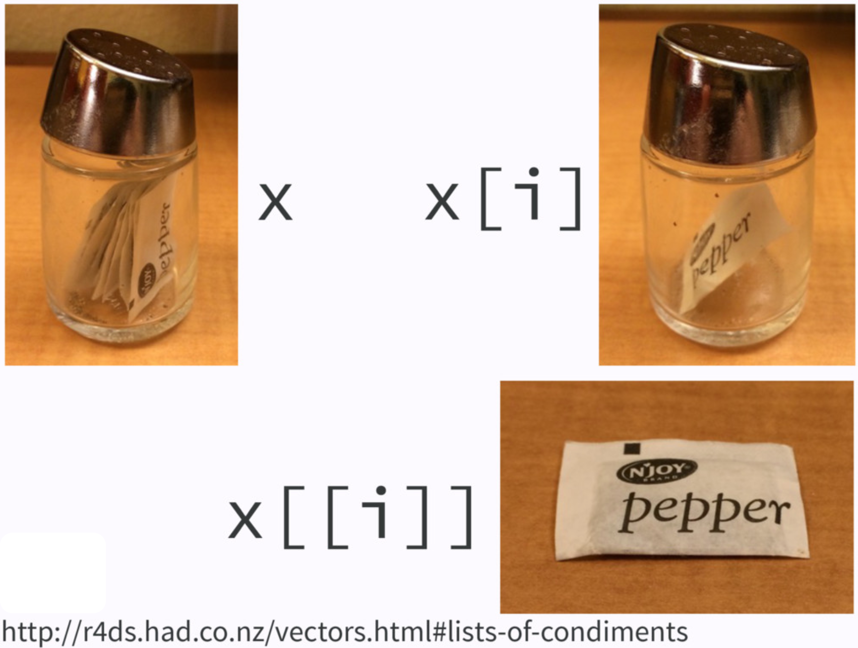

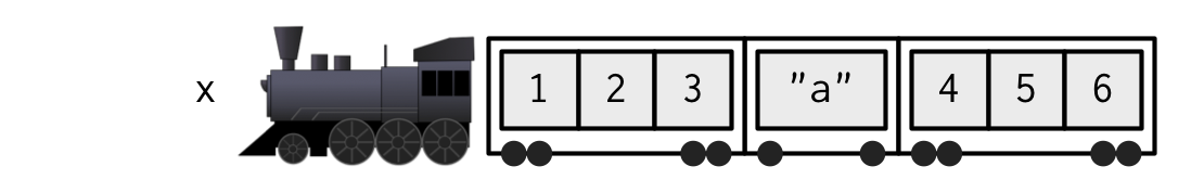
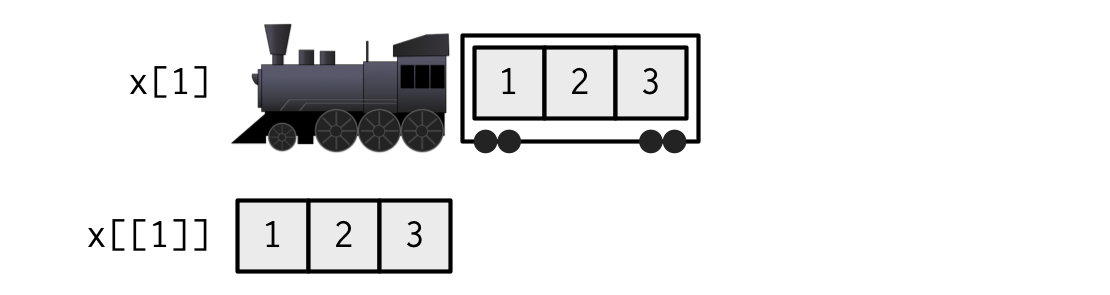
If list x is a train carrying objects, then x[[5]] is the object in car 5; x[4:6] is a train of cars 4-6.

— @RLangTip, https://twitter.com/RLangTip/status/268375867468681216

A.8 Data Structure - Matrix

• A matrix is a two-dimensional analog of a vector with attribute dim.

• Use command matrix() to create a matrix.

## Create a 3 by 2 matrix called mat
(mat <- matrix(data = 1:6, nrow = 3, ncol = 2)) 

     [,1] [,2]
[1,]    1    4
[2,]    2    5
[3,]    3    6

dim(mat); nrow(mat); ncol(mat)

[1] 3 2

[1] 3

[1] 2

# elements are arranged by row
matrix(data = 1:6, 
       nrow = 3, 
       ncol = 2, 
       byrow = TRUE) #<<

     [,1] [,2]
[1,]    1    2
[2,]    3    4
[3,]    5    6

attributes(mat)

$dim
[1] 3 2

A.8.1 Row and Column Names

mat

     [,1] [,2]
[1,]    1    4
[2,]    2    5
[3,]    3    6

## assign row names and column names
rownames(mat) <- c("A", "B", "C")
colnames(mat) <- c("a", "b")
mat

  a b
A 1 4
B 2 5
C 3 6

rownames(mat)

[1] "A" "B" "C"

colnames(mat)

[1] "a" "b"

attributes(mat)

$dim
[1] 3 2

$dimnames
$dimnames[[1]]
[1] "A" "B" "C"

$dimnames[[2]]
[1] "a" "b"

A.8.2 Subsetting a Matrix

• Use the same indexing approach as vectors on rows and columns.
• Use comma , to separate row and column index.
• mat[2, 2] extracts the element of the second row and second column.

mat

  a b
A 1 4
B 2 5
C 3 6

## all rows and 2nd column
## leave row index blank
## specify 2 in coln index
mat[, 2]

A B C 
4 5 6 

## 2nd row and all columns
mat[2, ] 

a b 
2 5 

## The 1st and 3rd rows and the 1st column
mat[c(1, 3), 1] 

A C 
1 3 

A.8.3 Binding Matrices

• cbind() (binding matrices by adding columns)

• rbind() (binding matrices by adding rows)

• When matrices are combined by columns (rows), they should have the same number of rows (columns).

mat

  a b
A 1 4
B 2 5
C 3 6

mat_c <- matrix(data = c(7,0,0,8,2,6), 
                nrow = 3, ncol = 2)
## should have the same number of rows
cbind(mat, mat_c)  

  a b    
A 1 4 7 8
B 2 5 0 2
C 3 6 0 6

mat_r <- matrix(data = 1:4, 
                nrow = 2, 
                ncol = 2)
## should have the same number of columns
rbind(mat, mat_r)  

  a b
A 1 4
B 2 5
C 3 6
  1 3
  2 4

A.9 Data Structure - Data Frame

• A data frame is of type list of equal-length vectors, having a 2-dimensional structure.

• More general than matrix: Different columns can have different types.

• Use data.frame() that takes named vectors as input “element”.

## data frame w/ an dbl column named age
## and char column named gender.
(df <- data.frame(age = c(19, 21, 40), 
                  gen = c("m","f", "m")))

  age gen
1  19   m
2  21   f
3  40   m

## a data frame has a list structure
str(df)  

'data.frame':   3 obs. of  2 variables:
 $ age: num  19 21 40
 $ gen: chr  "m" "f" "m"

## must set column names
## or they are ugly and non-recognizable
data.frame(c(19,21,40), c("m","f","m")) 

  c.19..21..40. c..m....f....m..
1            19                m
2            21                f
3            40                m

A.9.1 Properties of data frames

Data frame has properties of matrix and list.

names(df)  ## df as a list

[1] "age" "gen"

colnames(df)  ## df as a matrix

[1] "age" "gen"

length(df) ## df as a list

[1] 2

ncol(df) ## df as a matrix

[1] 2

dim(df) ## df as a matrix

[1] 3 2

## rbind() and cbind() can be used on df
df_r <- data.frame(age = 10, 
                   gen = "f")
rbind(df, df_r)

  age gen
1  19   m
2  21   f
3  40   m
4  10   f

df_c <- 
    data.frame(col = c("red","blue","gray"))
(df_new <- cbind(df, df_c))

  age gen  col
1  19   m  red
2  21   f blue
3  40   m gray

A.9.2 Subsetting a data frame

Can use either list or matrix subsetting methods.

df_new

  age gen  col
1  19   m  red
2  21   f blue
3  40   m gray

## Subset rows
df_new[c(1, 3), ]

  age gen  col
1  19   m  red
3  40   m gray

## select the row where age == 21
df_new[df_new$age == 21, ]

  age gen  col
2  21   f blue

## Subset columns
## like a list
df_new$age

[1] 19 21 40

df_new[c("age", "gen")]

  age gen
1  19   m
2  21   f
3  40   m

## like a matrix
df_new[, c("age", "gen")]

  age gen
1  19   m
2  21   f
3  40   m

df_new[c(1, 3), ]

  age gen  col
1  19   m  red
3  40   m gray

str(df["age"])  ## a data frame with one column

'data.frame':   3 obs. of  1 variable:
 $ age: num  19 21 40

str(df[, "age"])  ## becomes a vector by default

 num [1:3] 19 21 40

A.10 Special Objects

A.11 Plotting

A.11.1 Scatter plot

mtcars[1:15, 1:4]

                    mpg cyl  disp  hp
Mazda RX4          21.0   6 160.0 110
Mazda RX4 Wag      21.0   6 160.0 110
Datsun 710         22.8   4 108.0  93
Hornet 4 Drive     21.4   6 258.0 110
Hornet Sportabout  18.7   8 360.0 175
Valiant            18.1   6 225.0 105
Duster 360         14.3   8 360.0 245
Merc 240D          24.4   4 146.7  62
Merc 230           22.8   4 140.8  95
Merc 280           19.2   6 167.6 123
Merc 280C          17.8   6 167.6 123
Merc 450SE         16.4   8 275.8 180
Merc 450SL         17.3   8 275.8 180
Merc 450SLC        15.2   8 275.8 180
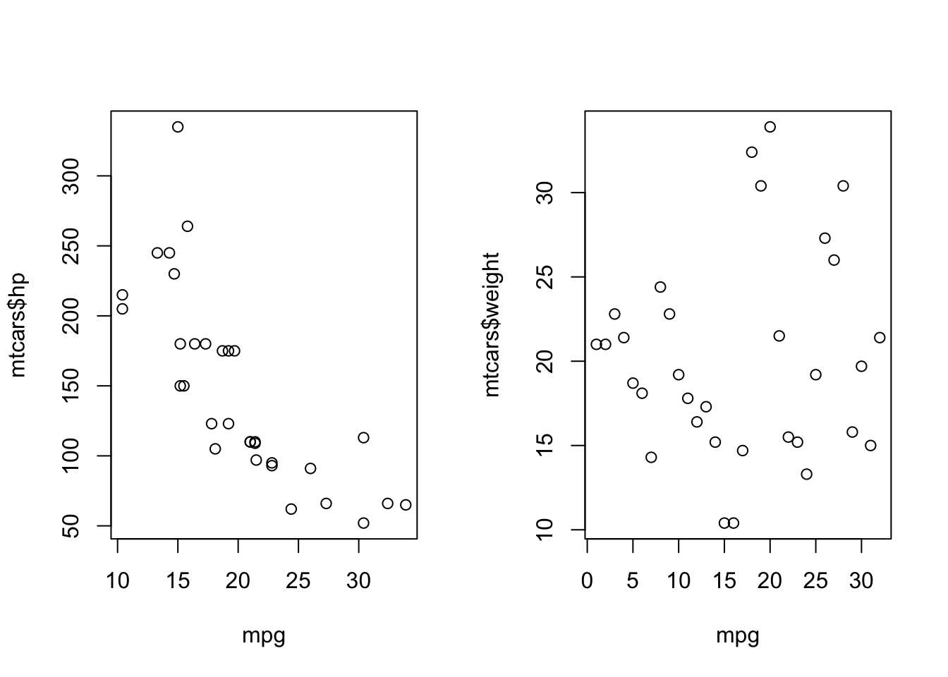
Cadillac Fleetwood 10.4   8 472.0 205

plot(x = mtcars$mpg, y = mtcars$hp, 
     xlab  = "Miles per gallon", 
     ylab = "Horsepower", 
     main = "Scatter plot", 
     col = "red", 
     pch = 5, las = 1)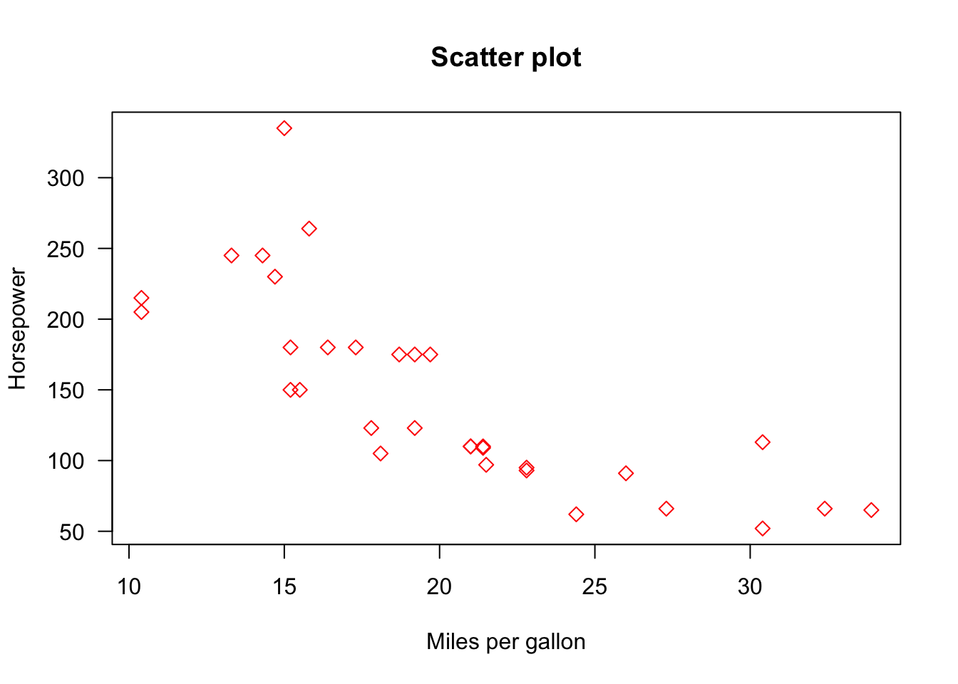

A.11.2 Argument pch

plot(x = 1:25, y = rep(1, 25), pch = 1:25, xlab = "", ylab = "", main = "pch", axes = FALSE)
axis(1, at = 1:25, cex.axis = 0.5)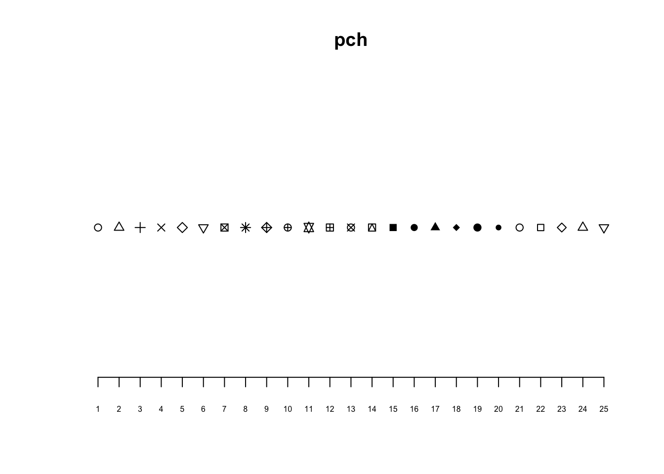

• The default is pch = 1

A.11.3 R Subplots

par(mfrow = c(1, 2))
plot(x = mtcars$mpg, y = mtcars$hp, xlab = "mpg")
plot(x = mtcars$mpg, y = mtcars$weight, xlab = "mpg")

A.11.4 Boxplot

par(mar = c(4, 4, 0, 0))
boxplot(mpg ~ cyl, 
        data = mtcars, 
        col = c("blue", "green", "red"), 
        las = 1, 
        horizontal = TRUE,
        xlab = "Miles per gallon", 
        ylab = "Number of cylinders")

A.11.5 Histogram

hist() decides the class intervals/with based on breaks. If not provided, R chooses one.

hist(mtcars$wt, 
     breaks = 20, 
     col = "#003366", 
     border = "#FFCC00", 
     xlab = "weights", 
     main = "Histogram of weights",
     las = 1)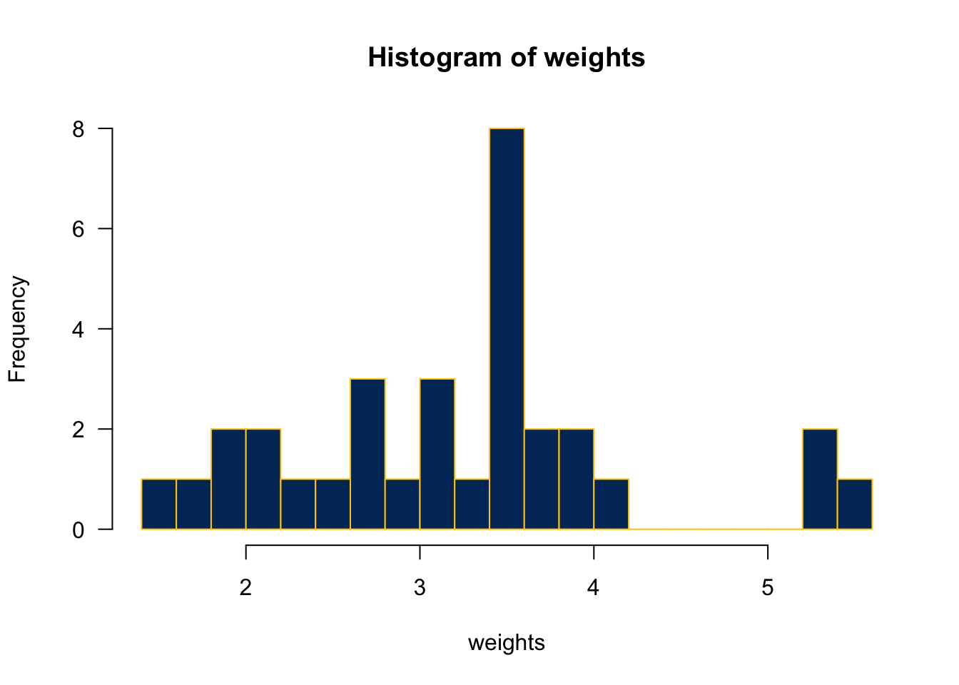

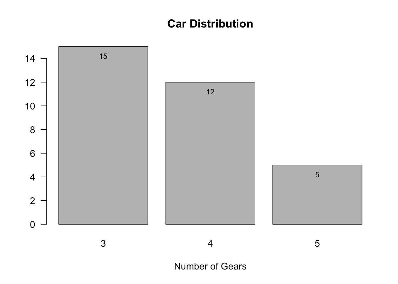
• Besides color names, you can also use hex number to specify colors. Pretty handy.

A.11.6 Barplot

(counts <- table(mtcars$gear)) 

 3  4  5 
15 12  5 

my_bar <- barplot(counts, 
                  main = "Car Distribution", 
                  xlab = "Number of Gears", 
                  las = 1)
text(x = my_bar, y = counts - 0.8, 
     labels = counts, 
     cex = 0.8)

A.11.7 Pie chart

• Pie charts are used for categorical variables, especially when we want to know percentage of each category.

• The first argument is the frequency table, and you can add labels to each category.

(percent <- round(counts / sum(counts) * 100, 2))

    3     4     5 
46.88 37.50 15.62 

(labels <- paste0(3:5, " gears: ", percent, "%"))

[1] "3 gears: 46.88%" "4 gears: 37.5%"  "5 gears: 15.62%"

pie(x = counts, labels = labels,
    main = "Pie Chart", 
    col = 2:4, 
    radius = 1)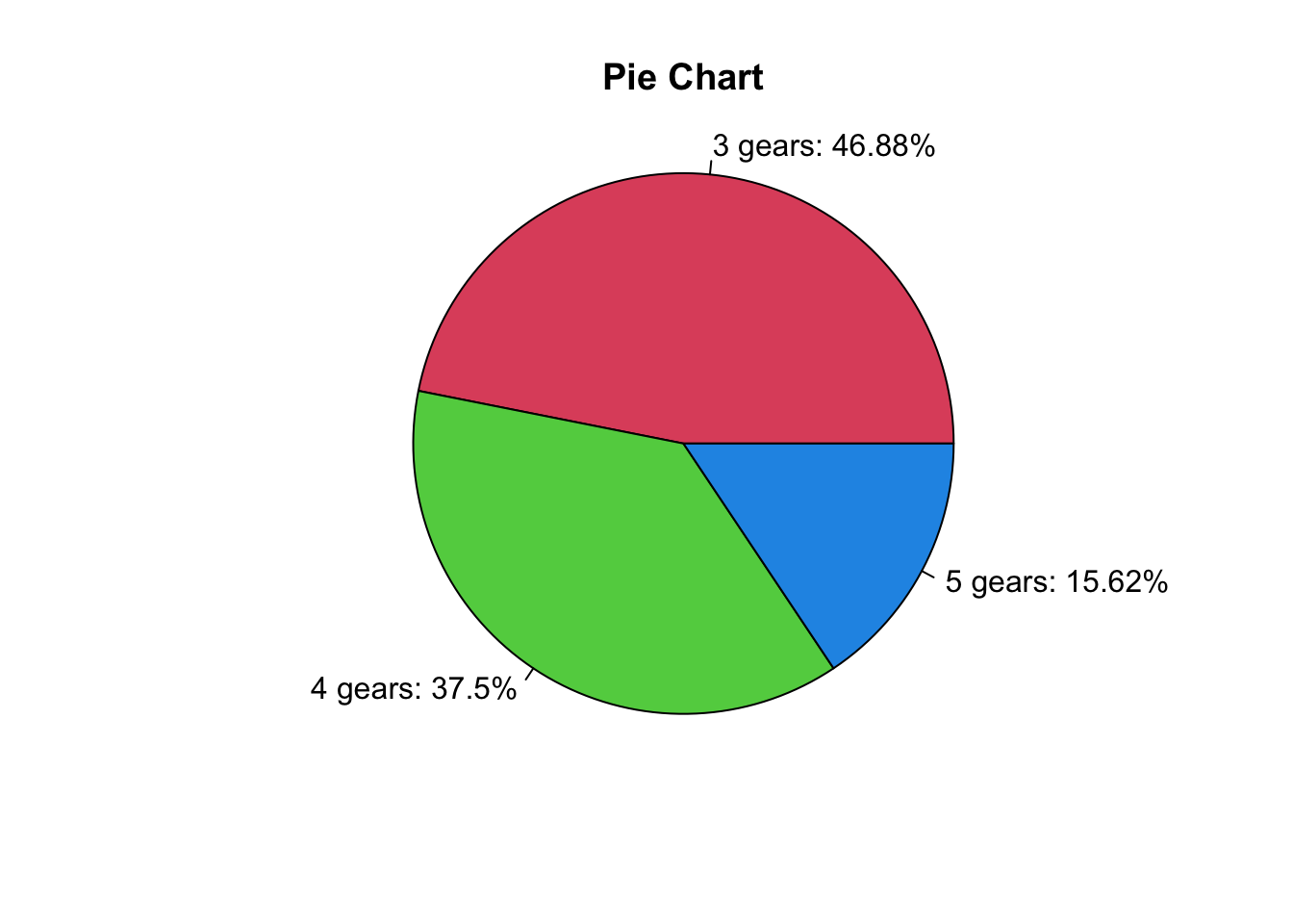

A.11.8 2D imaging

• The image() function displays the values in a matrix using color.

matrix(1:30, 6, 5)

     [,1] [,2] [,3] [,4] [,5]
[1,]    1    7   13   19   25
[2,]    2    8   14   20   26
[3,]    3    9   15   21   27
[4,]    4   10   16   22   28
[5,]    5   11   17   23   29
[6,]    6   12   18   24   30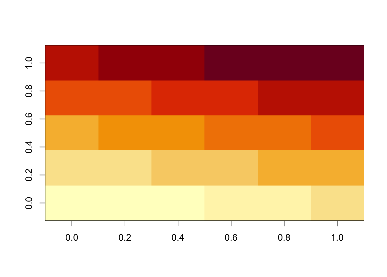

image(matrix(1:30, 6, 5))

library(fields)

Loading required package: spam

Spam version 2.10-0 (2023-10-23) is loaded.
Type 'help( Spam)' or 'demo( spam)' for a short introduction 
and overview of this package.
Help for individual functions is also obtained by adding the
suffix '.spam' to the function name, e.g. 'help( chol.spam)'.

Attaching package: 'spam'

The following objects are masked from 'package:base':

    backsolve, forwardsolve

Loading required package: viridisLite

Try help(fields) to get started.

str(volcano)

 num [1:87, 1:61] 100 101 102 103 104 105 105 106 107 108 ...

image.plot(volcano)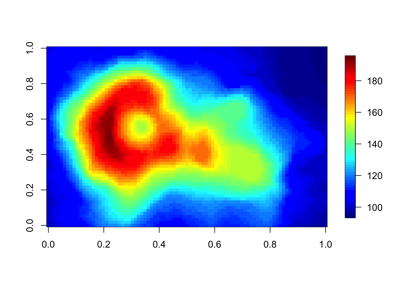

x <- 10*(1:nrow(volcano))
y <- 10*(1:ncol(volcano))
image(x, y, volcano, col = hcl.colors(100, "terrain"), axes = FALSE)
contour(x, y, volcano, levels = seq(90, 200, by = 5),
        add = TRUE, col = "brown")
axis(1, at = seq(100, 800, by = 100))
axis(2, at = seq(100, 600, by = 100))
box()
title(main = "Maunga Whau Volcano", font.main = 4)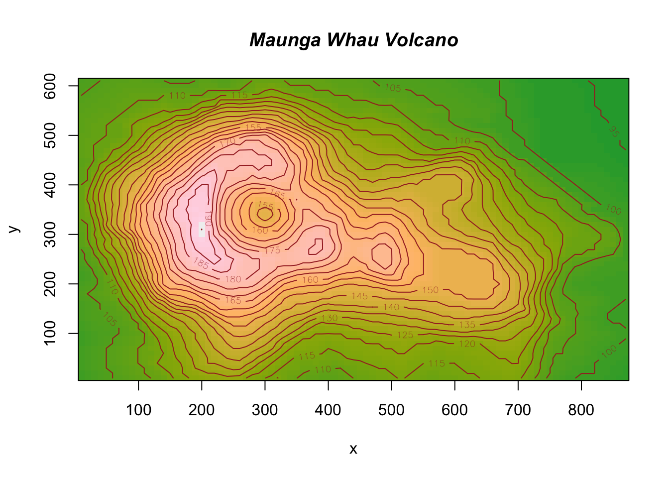

A.11.9 3D scatter plot

library(scatterplot3d)
scatterplot3d(x = mtcars$wt, y = mtcars$disp, z = mtcars$mpg, 
              xlab = "Weights", ylab = "Displacement", zlab = "Miles per gallon", 
              main = "3D Scatter Plot",
              pch = 16, color = "steelblue")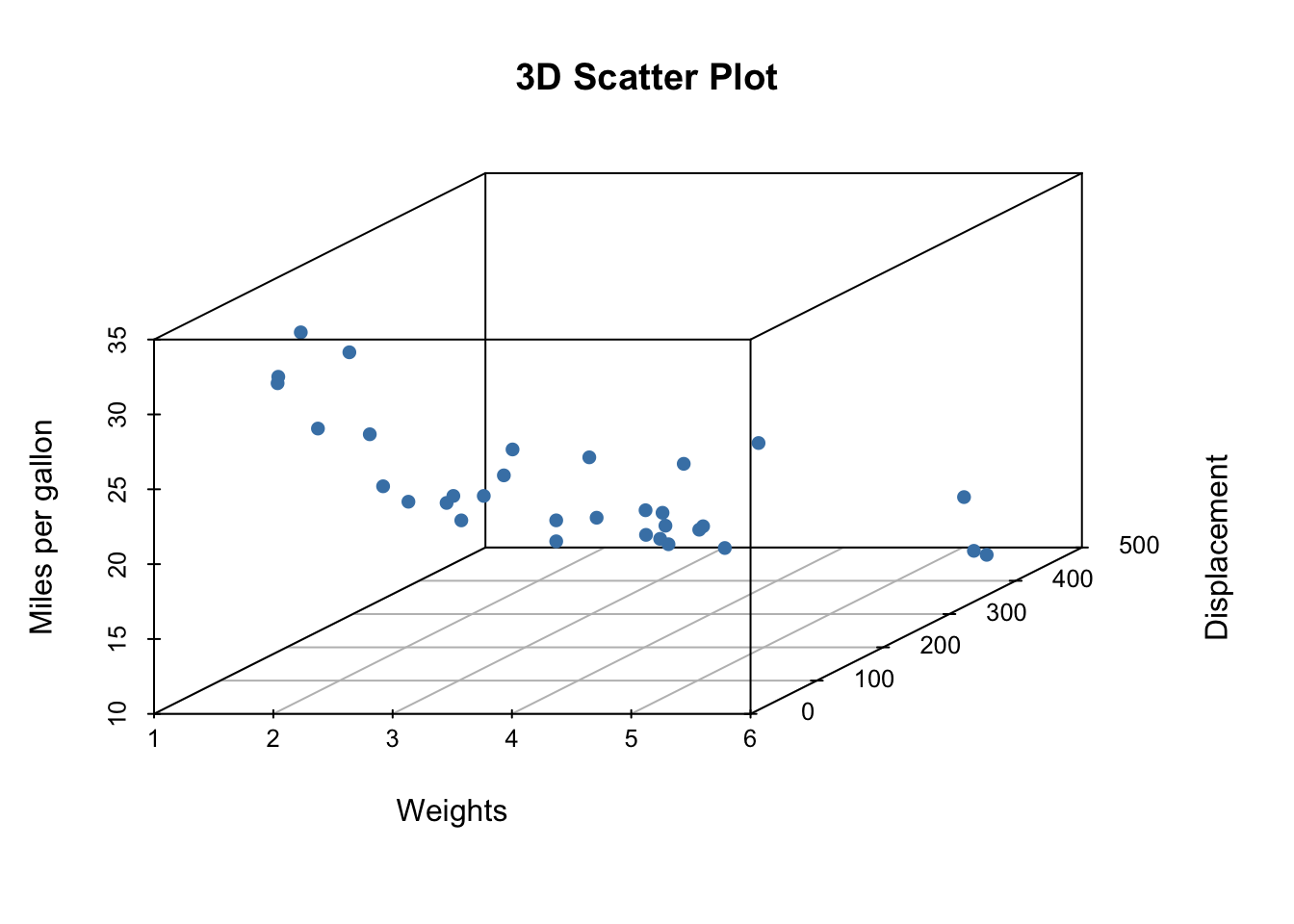

A.11.10 Perspective plot

# Exaggerate the relief
z <- 2 * volcano      
# 10 meter spacing (S to N)
x <- 10 * (1:nrow(z))   
# 10 meter spacing (E to W)
y <- 10 * (1:ncol(z))   
par(bg = "slategray")
persp(x, y, z, theta = 135, phi = 30, col = "green3", scale = FALSE,
      ltheta = -120, shade = 0.75, border = NA, box = FALSE)

A.12 Special Objects

A.12.1 NA

• NA means Not Available, which is a logical constant of length 1 for a missing value indicator.

• Each type of vector has its own missing value. They all are reserved words.

• You can always use NA and it will be converted to the correct type.

NA            # logical

[1] NA

NA_integer_   # integer

[1] NA

NA_real_      # double

[1] NA

NA_character_ # character

[1] NA

## The NA in the vector x is NA_real_
x <- c(NA, 0, 1)
typeof(x)  

[1] "double"

is.na(x)

[1]  TRUE FALSE FALSE

A.12.2 NULL

• NULL represents the null object, an object representing nothing.
• NULL is a reserved word and can also be the product of importing data with unknown data type.
• NULL typically behaves like a vector of length 0.

y <- c(NA, NULL, "")
y

[1] NA ""

## only first element is evaluated...
is.null(y) 

[1] FALSE

## a missing value is a value we don't know.
## It is something.
is.null(NA)

[1] FALSE

is.null(NULL)

[1] TRUE

# empty character is something, not nothing!
is.null("")

[1] FALSE

A.12.3 NaN, Inf, and -Inf

• Integers have one special value: NA, while doubles have four: NA, NaN, Inf and -Inf.

• NaN means Not a Number.

• All three special values NaN, Inf and -Inf can arise during division.

c(-1, 0, 1) / 0

[1] -Inf  NaN  Inf

• Avoid using ==. Use functions is.finite(), is.infinite(), and is.nan().

is.finite(0)

[1] TRUE

is.nan(0/0)

[1] TRUE

is.infinite(7.8/1e-307)

[1] FALSE

is.infinite(7.8/1e-308)

[1] TRUE

A.12.4 Helper Functions

• NaN is a missing value too.

• There should be something there, but it’s Not Available to us because of invalid operation.

	0	Inf	NA	NaN
is.finite()	v
is.infinite()		v
is.na()			v	v
is.nan()				v

A.12.5 NA, NULL, NaN comparison

class(NULL); class(NA); class(NaN)

[1] "NULL"

[1] "logical"

[1] "numeric"

NULL > 5; NA > 5; NaN > 5

logical(0)

[1] NA

[1] NA

length(NULL); length(NA); length(NaN)

[1] 0

[1] 1

[1] 1

(vx <- c(3, NULL, 5)); (vy <- c(3, NA, 5)); (vz <- c(3, NaN, 5))

[1] 3 5

[1]  3 NA  5

[1]   3 NaN   5

sum(vx)  # NULL isn't a problem cuz it doesn't exist

[1] 8

sum(vy)

[1] NA

sum(vy, na.rm = TRUE)

[1] 8

sum(vz)

[1] NaN

sum(vz, na.rm = TRUE)

[1] 8

A.13 Conditions

# The condition must evaluate to either TRUE or FALSE.
if (condition) {
  # code executed when condition is TRUE
} else {
  # code executed when condition is FALSE
}

if (c(TRUE, FALSE)) {}
#> Warning in if (c(TRUE, FALSE)) {: the condition has length > 1 and only the
#> first element will be used
#> NULL

if (NA) {}
#> Error in if (NA) {: missing value where TRUE/FALSE needed

• You can use || (or) and && (and) to combine multiple logical expressions.

if (cond1 || cond2) {
  # code executed when condition is TRUE
}

• The basic If-else statement structure is that we write if then put a condition inside a pair of parenthesis, then use curly braces to wrap the code to be run when the condition is TRUE.

• If we want to have the code to be run when the condition is FALSE, we add else and another pair of curly braces.

• curly braces is not necessary if you just have one line of code to be run.

• The condition must evaluate to either one TRUE or one FALSE.

• If it’s a vector, you’ll get a warning message, and only the first element will be used.

• If it’s an NA, you’ll get an error.

if (this) {
    # do that
} else if (that) {
    # do something else
} else {
    # 
}

if (celsius <= 0) {
    "freezing"
} else if (celsius <= 10) {
    "cold"
} else if (celsius <= 20) {
   "cool"
} else if (celsius <= 30) {
    "warm"
} else {
    "hot"
}

• If we want to have multiple conditions, we add the word else if.

• The code below is an example of converting numerical data to categorical data, freezing, cold, warm and hot.

• It’s not the best way to do conversion.

• If you end up with a very long series of chained if-else statements, rewrite it!

https://speakerdeck.com/jennybc/code-smells-and-feels

• If you end up with a very long series of chained if-else statements, rewrite it! Don’t confuse readers and especially yourself.
• We have a function called “get same data”.
• When you read the code in a linear fashion from top to bottom, you are falling down and down into conditions that were like a long time ago that you saw what you are actually checking.
• Here is another way to write the exactly the same function. ….. and now I am on the happy path. I get the data.
• So if I open a file, and I know that something is gone wrong and checking all these things, I am much happier to be facing this than that!
• I think our brain cannot process too many layers. When we are trying to analyze so many layers, we just get lost.

https://speakerdeck.com/jennybc/code-smells-and-feels

• So there is no else, there is only if!
• Back, on the left, every if has an else.
• On the right, we have no else. And this makes your code much more readable!

A.14 Functions

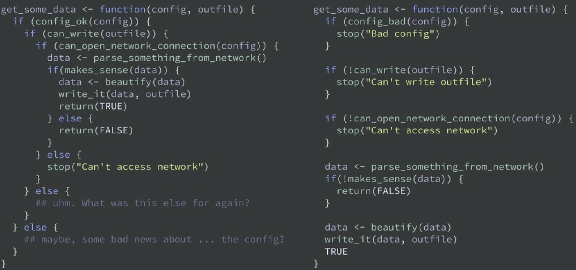
• Write a function whenever you’ve copied and pasted your code more than twice.

• Three key steps/components:

  • pick a name for the function.
  • list the inputs, or arguments, to the function inside function.
  • place the code you have developed in body of the function.

function_name <- function(arg1, arg2, ...) {
    ## body
    return(something)
}

add_number <- function(a, b) {
    c <- a + b
    return(c)
}

n1 <- 9
n2 <- 18
add_number(n1, n2)

[1] 27

A.15 Loops

A.15.1 for loops

## Syntax
for (value in that) {
    this
}

for (i in 1:5) {
    print(i)
}

[1] 1
[1] 2
[1] 3
[1] 4
[1] 5

for (x in c("My", "1st", "for", "loop")) {
    print(x)
}

[1] "My"
[1] "1st"
[1] "for"
[1] "loop"

A.15.2 while loops

while (condition) {
    # body
}

• You can rewrite any for loop as a while loop, but you can’t rewrite every while loop as a for loop.

for (i in seq_along(x)) {
    # body
}

# Equivalent to
i <- 1
while (i <= length(x)) {
    # body
    i <- i + 1 
}

• We find how many tries it takes to get 5 heads in a row:

## a function that sample one from "T" or "H"
flip <- function() sample(c("T", "H"), 1)

flips <- 0; nheads <- 0

while (nheads < 5) {
    if (flip() == "H") {
        nheads <- nheads + 1
    } else {
        nheads <- 0
    }
    flips <- flips + 1
}

flips

[1] 5