14  Point and Interval Estimation

In this chapter we will be talking about estimation including point and interval estimation. Point estimation uses one single number computed from the sample to estimate our unknown parameter. Interval estimation provides uncertainty quantification and uses a range of plausible numbers to let us know where the truth unknown parameter may be located.

14.1 Point Estimator

Let me ask you a question.

If you could only use a single number to guess the unknown population mean, $\mu$, what number would you like to use?

If the single number you use can be computed from of sample data $(X_1,X_2,\dots ,X_n)$, then you use a point estimator to estimate the unknown parameter $\mu$. Previously we learned that a sample statistic is any transformation or function of $(X_1,X_2,\dots ,X_n)$. Therefore, any statistic is considered a point estimator if it is used to estimate a population parameter.

A point estimate is a value of a point estimator used to estimate a population parameter. So here is the subtle difference. A point estimator is a random variable which is a function of sample data $(X_1,X_2,\dots ,X_n)$ (before actually being collected), and a point estimate is the realized value a point estimator, which is a value calculated from the collected data. For example, $\bar{X}=\frac{1}{n}\sum _{i=1}^n{X}_i$ is a point estimator, and with the sample data $(x_1,x_2,x_3)=(2,3,7)$, the point estimate is $\bar{x}=\frac{1}{3}\sum _{i=1}^3{x}_i=\frac{1}{3}(2+3+7)=4.$

Back to the question. If we want to estimate the unknown population mean, which number we use to estimate it? We now have an intuitive answer. The sample mean $\bar{X}$ is a statistic and a point estimator for the population mean $\mu$.

---

Sample Mean as an Point Estimator

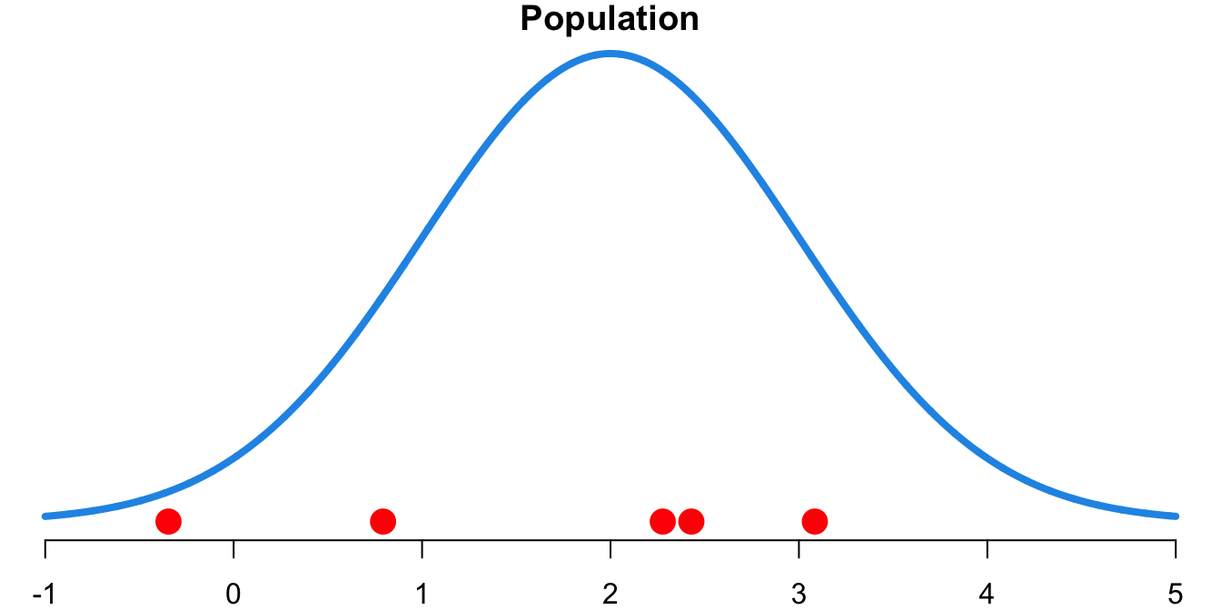
Let’s see how the sample mean is used as an point estimator for $\mu .$ Suppose the true population distribution is $N(2,1)$. Here the population mean $\mu$ is two, but let’s pretend we don’t know its value and see how the sample mean performs. Such analysis is called simulation study.

We are going to collect a sample of size five, $(x_1,x_2,x_3,x_4,x_5)$. In the simulation, we draw five values from $N(2,1)$. The five drawn values are treated as our sample data, and $N(2,1)$ is the population distribution. In R, we use rnorm() to generate random numbers from a normal distribution, where the first argument is the number of observations to be generated.

## Generate data x1, x2, x3, x4, x5, each from distribution N(2, 1)
set.seed(1234)
x_data_1 <- rnorm(n = 5, mean = 2, sd = 1)

The following shows the realized five data points and the sample mean.

x1	x2	x3	x4	x5	sample mean
0.79	2.28	3.08	-0.35	2.43	1.65

Here we use the sample mean $\bar{X}=\frac{1}{5}\sum _{i=1}^5{X}_i$ as our point estimator for $\mu$, and given the sample, the point estimate is $\bar{x}=$ 1.65. You can see that the true $\mu$ is two, but the point estimate $\bar{x}$ is not equal to $\mu$. Why?

As we discussed in ?sec-prob-samdist, due to the randomness nature of drawing a sample value from the population distribution, we do not expect the statistic to be the same as the corresponding parameter. It is possible that most of our sample values happen to be larger or smaller than the true mean, or we may unluckily get an outlier sample value that distorts and drags the sample value toward it. In such cases, the sample mean will be not close to the true population mean. You can think this way. One data point represents one piece of information about the unknown population distribution. With a small sample size, our sample only represents a small part of the unknown distribution. The gap between sample mean and the true population mean is kind of like information lost because of not being able to collect the rest of the subjects in the population.

Figure 14.1 shows the sample data and the population distribution $N(2,1)$. Notice that we have an extreme value $-0.35$ that is two standard deviations below the mean, and this causes the sample mean to be small.

Figure 14.1: Population distribution and sample data.

Well, we could collect a sample again if resources are permitted. In simulation, another sample of size five is drawn from the same population $N(2,1)$, and the result is shown below.

x1	x2	x3	x4	x5	sample mean
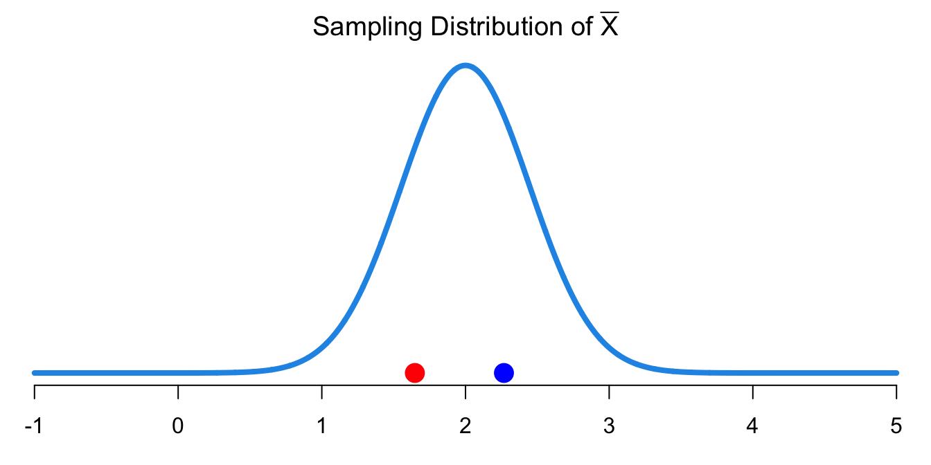
2.59	2.71	1.89	1.55	2.61	2.27

The second sample mean, $\bar{x}=$ 2.27, is different from the first one. Why do the first sample and the second sample give us different sample means? Now you see why we want to learn sampling distribution. We use sample mean as the point estimator for $\mu$, and the sample mean has its own sampling distribution. Therefore, the sample mean varies from sample to sample due to its randomness nature.

We have connected sampling distribution to statistical inference, in particular the point estimation together. Figure 14.2 shows the sampling distribution of $\bar{X}$ which is $N(2,1/5)$ and the two sample mean values calculated from the two data sets. Now can you see why we want to use $\bar{X}$ as the point estimator for $\mu$? It is because the expected value of $\bar{X}$, $E(\bar{X})$ is exactly equal to $\mu$, meaning that if we were able to produces a lot of $\bar{x}$s, the average of these $\bar{x}$s will be very close to the true unknown $\mu$ although single one $\bar{x}$ may still be distant from $\mu$. When the expected value of a point estimator is equal to the parameter it estimates, we say it is an unbiased estimator. Therefore, the sample mean $\bar{X}$ is an unbiased estimator for the population mean $\mu$ because $E(\bar{X})=\mu$.

Figure 14.2: Sampling Distribution of Sampling Mean.

---

Why Point Estimates Are Not Enough

If you want to estimate $\mu$, would you prefer to report a range of values the parameter might be in or a single estimate like $\bar{x}$?

Since $\bar{X}$ is random and has its own distribution, its value varies from sample to sample. However, in reality we usually have only one data set, and one realized sample mean, and we are not able to replicate other data sets due to limited resources. We don’t know the sample mean we got is close to the true unknown population mean or not. First, the sample mean can go anywhere of its distribution, and the one we got may be far away from $\mu$. Moreover, we don’t know the value of $\mu$! It does not make much sense to use just one single number when those uncertainty are there.

If you want to catch a fish, would you prefer to use a spear or a net? I would use a net because I’m not a sharpshooter, and using a net covers a large range of possible locations where the fish can be. Due to the variation of $\bar{X}$, if we report a point estimate, we probably won’t hit the exact population parameter. If we report a range of plausible values, we have a good shot at capturing the parameter.

14.2 Confidence Intervals

In statistics, a plausible range of values for $\mu$ is called a confidence interval (CI). This range depends on how precise and reliable our statistic is as an estimate of the parameter. To construct a CI for $\mu$, we first need to quantify the variability of our sample mean. Quantifying this uncertainty requires a measurement of how much we would expect the sample statistic to vary from sample to sample. This is in fact the variance of the sampling distribution of the sample mean! Intuitively speaking, if $\bar{x}$ varies a lot, we are more uncertain about whether the $\bar{x}$ we got is close to the $\mu$ or not. In other words, the precision of the estimation is not that good. In order to make sure that the plausible range of values does capture $\mu$, we need to include more possible values, and make the range larger. Do we know the variance of $\bar{X}$? Absolutely. Thanks to CLT, $\bar{X}\sim N(\mu ,{\sigma }^2/n)$ regardless of what the population distribution is.

How confident we are about the CI covering the parameter is called the level of confidence. The higher the confidence level is, the more reliable the CI is because the CI is more likely to capture the parameter.

Note

Given the same level of confidence, the larger the variation of $\bar{X}$ is, the wider the CI for $\mu$ will be.

---

Precision vs. Reliability

With a fixed sample size, the precision and reliability of a confidence interval are trading off. Here is a question.

If we want to be very certain that we capture $\mu$, should we use a wider or a narrower interval? What drawbacks are associated with using a wider interval?

We use a wider interval because a wider interval is more likely to capture the population parameter value. So a more reliable confidence interval is wider than a less reliable confidence interval. But What drawbacks are associated with using a wider interval?

The precision and reliability trade-off is clearly explained in the cute comic in Figure 14.3. I can say I am 100% confident that your exam 1 score is between 0 and 100. Am I right? Yes. But do I provide helpful information? Absolutely not, the interval includes every possible score of the exam. The interval is too wide to be helpful. Such interval is 100% reliable but with no precision at all.

Figure 14.3: Balance between precision and reliability. Source: https://thestatsninja.com/2019/02/19/how-to-navigate-confidence-intervals-with-confidence/

Narrower intervals are more precise but less reliable, while wider intervals are more reliable but less precise. How can we get best of both worlds – high precision and high reliability/accuracy, meaning short interval with high level of confidence? What we need is larger sample size, given that the sample quality is good. It is a quite easy statement, but sometimes it’s hard to collect more samples.

---

A Confidence Interval Is for a Parameter

A confidence interval is for a parameter, NOT a statistic. Remember, a confidence interval is a way of doing estimation for a unknown parameter. For example, we use the sample mean to form a confidence interval for the population mean.

We NEVER say “The confidence interval of the sample mean, $\bar{X}$, is ….” We SAY “The confidence interval for the true population mean $\mu$, is …”

In general, a confidence interval for $\mu$ has the form

$\bar{x}\pm m=(\bar{x}-m,\bar{x}+m)$

The $m$ is called the margin of error. It controls the width of the interval $2m$. The CI is centered at the sample mean, and $\bar{x}-m$ is the lower bound and $\bar{x}+m$ is the upper bound of the confidence interval. The point estimate, $\bar{x}$, and margin of error, $m$, can be obtained from known quantities and our data once sampled.

---

$(1-\alpha )100\mathrm{\%}$ Confidence Intervals

Formally, for $0\le \alpha \le 1$, we define the confidence level $1-\alpha$ as the proportion of times that the CI contains the population parameter, assuming that the estimation process is repeated a large number of times.

The confidence level can be any number between zero and one. Common choices for the confidence level include 90% $(\alpha =0.10)$, 95% $(\alpha =0.05)$ and 99% $(\alpha =0.01)$. Keep in mind that confidence level tells us the reliability of the interval. Because precision and reliability have a trade-off relationship, a CI with very high confidence level (high reliability) will have less precision, i.e., larger margin of error and with width of the interval. 95% is the most common level because it has a good balance between precision (width of the CI) and reliability (confidence level).

• High reliability and Low precision: I am 100% confident that the mean height of Marquette students is between 3’0” and 8’0”.
  • Duh…🤷
• Low reliability and High precision: I am 20% confident that mean height of Marquette students is between 5’6” and 5’7”.
  • This is far from the truth… 🙅

---

$95\mathrm{\%}$ Confidence Intervals for $\mu$

We’ve learned the general form of a confidence interval for $\mu$ and defined the confidence level. We now formally derive the form of the $(1-\alpha )100\mathrm{\%}$ confidence interval for $\mu$. For simplicity, here we assume $\sigma$ is known to us when the interval is constructed. A confidence interval can be derived from the sampling distribution of the point estimator. Such approach is called the distribution-based approach. A confidence interval can also be derived using simulation, and such approach is called simulation-based approach, bootstraping method for example. This chapter we build a CI based on the sampling distribution of $\bar{X}$. We discuss bootstraping in Chapter 15.

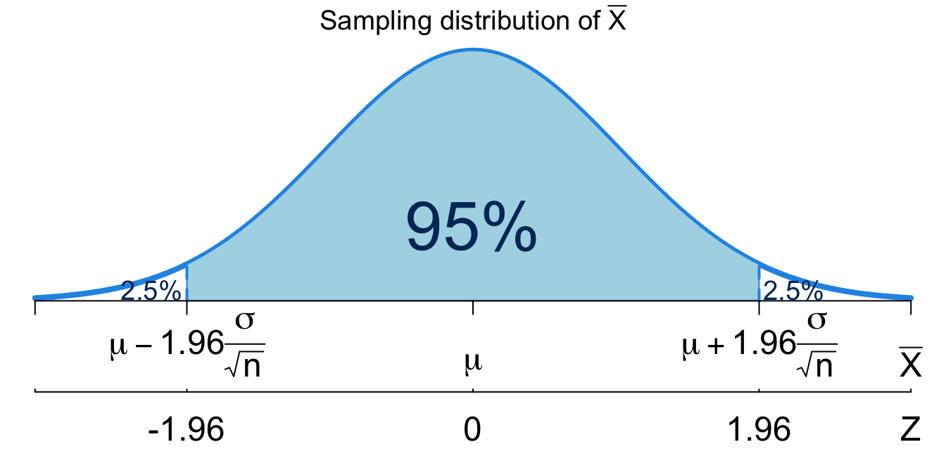
Suppose we want to obtain the $95\mathrm{\%}$ confidence interval for $\mu$. So $\alpha =0.05$. We start with the sampling distribution of $\bar{X}\sim N(\mu ,\frac{{\sigma }^2}{n})$ shown in Figure 14.4. The sampling distribution tells us that the realized value $\bar{x}$ will be within 1.96 SDs of the population mean, $\mu$, $95\mathrm{\%}$ of the time. In other words,

$$P(\mu -1.96\frac{\sigma }{\sqrt{n}}<\bar{X}<\mu +1.96\frac{\sigma }{\sqrt{n}})=0.95$$

Here the $z$-score of 1.96 is the 97.5% percentile of the standard normal distribution and -1.96 is the 2.5% percentile. The $z$-score 1.96 is associated with 2.5% area to the right and is called a critical value denoted as $z_{0.025}=z_{\alpha /2}$ . The $z$-score -1.96 is associated with 2.5% area to the left, and it happens to be the negative value of $z_{0.025}$ because of the symmetry of normal distribution.

Figure 14.4: Sampling distribution of the sample mean with 95% probability in the middle.

We learned that $$P(\mu -1.96\frac{\sigma }{\sqrt{n}}<\bar{X}<\mu +1.96\frac{\sigma }{\sqrt{n}})=0.95.$$ The probability that the variable $\bar{X}$ is in the interval $(\mu -1.96\frac{\sigma }{\sqrt{n}},\mu +1.96\frac{\sigma }{\sqrt{n}})$ is 95%. But is the interval $(\mu -1.96\frac{\sigma }{\sqrt{n}},\mu +1.96\frac{\sigma }{\sqrt{n}})$ our confidence interval?

The answer is No ❌! Remember that we don’t know $\mu$ and we are estimating it. The interval cannot be determined because it involves the unknown quantity $\mu$. But don’t be too disappointed. We are almost there.

We can arrange the inequality in the probability so that $\mu$ is in the middle and the probability remains unchanged.

• $$\mu -1.96\frac{\sigma }{\sqrt{n}}<\bar{X}⟺\mu <\bar{X}+1.96\frac{\sigma }{\sqrt{n}}$$

• $$\bar{X}<\mu +1.96\frac{\sigma }{\sqrt{n}}<⟺\bar{X}-1.96\frac{\sigma }{\sqrt{n}}<\mu$$

• $$\mu -1.96\frac{\sigma }{\sqrt{n}}<\bar{X}<\mu +1.96\frac{\sigma }{\sqrt{n}}⟺\bar{X}-1.96\frac{\sigma }{\sqrt{n}}<\mu <\bar{X}+1.96\frac{\sigma }{\sqrt{n}}$$

$$\begin{array}{r}P(\mu -1.96\frac{\sigma }{\sqrt{n}}<\bar{X}<\mu +1.96\frac{\sigma }{\sqrt{n}})=P\left(\boxed{{\displaystyle \bar{X}-1.96\frac{\sigma }{\sqrt{n}}<\mu <\bar{X}+1.96\frac{\sigma }{\sqrt{n}}}}\right)=0.95\end{array}$$

We are done! With sample data of size $n$, $(\bar{x}-1.96\frac{\sigma }{\sqrt{n}},\bar{x}+1.96\frac{\sigma }{\sqrt{n}})$ is our $95\mathrm{\%}$ CI for $\mu$. Note that if $\sigma$ is known to us, the interval can be computed from our data because we know the sample size, and we can get the sample mean. The margin of error $m=1.96\frac{\sigma }{\sqrt{n}}$.

14.3 Confidence Intervals for $\mu$ When $\sigma$ is Known

We just obtained the 95% confident interval for $\mu$. How about the general $(1-\alpha )100$ confident interval for $\mu$ (when $\sigma$ is known)? We first introduce the requirements for constructing the interval, then provide the interval formula.

The requirements for estimating $\mu$ when $\sigma$ is known include

• 👉 The sample should be a random sample, such that all data $X_i$ are drawn from the same population and $X_i$ and $X_j$ are independent. In fact, any methods in this course are based on the assumption of a random sample
• 👉 The population standard deviation, $\sigma$, is known.
• 👉 The population is either normally distributed, $n>30$ or both, i.e., $X_i\sim N(\mu ,{\sigma }^2)$. The sample size $n>30$ allows the central limit theorem to be applied and hence normality is satisfied.

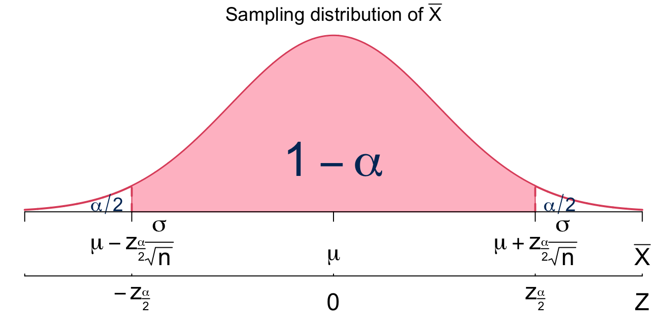
The general $(1-\alpha )100\mathrm{\%}$ confidence interval for $\mu$ can be borrowed from the $95\mathrm{\%}$ confidence interval for $\mu$, $(\bar{x}-z_{0.025}\frac{\sigma }{\sqrt{n}},\bar{x}+z_{0.025}\frac{\sigma }{\sqrt{n}})$. The 95% confidence level means $\alpha =0.05$. For the general $(1-\alpha )100\mathrm{\%}$ confidence interval, we just replace $z_{0.025}$ with $z_{\alpha /2}$ for any $\alpha$ between zero and one. Therefore, the general $(1-\alpha )100\mathrm{\%}$ confidence interval for $\mu$ is

To sum up, we provide procedures for constructing a confidence interval for $\mu$ when $\sigma$ is known:

1. Check that the requirements are satisfied.

2. Decide $\alpha$ or the confidence level $(1-\alpha )$.

3. Find the critical value, $z_{\alpha /2}$.

4. Evaluate margin of error, $m=z_{\alpha /2}\cdot \frac{\sigma }{\sqrt{n}}$.

5. Construct the $(1-\alpha )100\mathrm{\%}$ CI for $\mu$ using the sample mean, $\bar{x}$, and margin of error, $m$:

$$\boxed{{\displaystyle \bar{x}\pm z_{\alpha /2}\frac{\sigma }{\sqrt{n}}\text{ or }(\bar{x}-z_{\alpha /2}\frac{\sigma }{\sqrt{n}},\bar{x}+z_{\alpha /2}\frac{\sigma }{\sqrt{n}})}}$$

---

Example

Suppose we want to know the mean systolic blood pressure (SBP) of a population. Assume that the population distribution is normal and has a standard deviation of 5 mmHg. We have a random sample of 16 subjects from this population with a mean of 121.5 mmHg. Estimate the mean SBP with a 95% confidence interval.

We construct the confidence interval step by step using the procedure.

1. Requirements:
   • Normality is assumed, $\sigma =5$ is known and a random sample is collected.
2. Decide $\alpha$:
   • $\alpha =0.05$
3. Find the critical value $z_{\alpha /2}$:
   • $z_{\alpha /2}=z_{0.025}=1.96$
4. Evaluate margin of error $m=z_{\alpha /2}\frac{\sigma }{\sqrt{n}}$:
   • $m=(1.96)\frac{5}{\sqrt{16}}=2.45$
5. Construct the $(1-\alpha )100\mathrm{\%}$ CI:
   • The 95% CI for the mean SBP is $\bar{x}\pm z_{\alpha /2}\frac{\sigma }{\sqrt{n}}=(121.5-2.45,121.5+2.45)=(119.05,123.95)$

Below is a demonstration of how to find the 95% CI for SBP using R/Python

R

## save all information we have
alpha <- 0.05
n <- 16
x_bar <- 121.5
sig <- 5

## 95% CI
## z-critical value
(cri_z <- qnorm(p = alpha / 2, lower.tail = FALSE))  
# [1] 1.96

## margin of error
(m_z <- cri_z * (sig / sqrt(n)))  
# [1] 2.45

## 95% CI for mu when sigma is known
x_bar + c(-1, 1) * m_z  
# [1] 119 124

Python

import numpy as np
from scipy.stats import norm
import matplotlib.pyplot as plt

# Given values
alpha = 0.05
n = 16
x_bar = 121.5
sig = 5  # Population standard deviation

# z-critical value
cri_z = norm.ppf(1 - alpha / 2)
cri_z
# 1.959963984540054

cri_z = norm.isf(alpha / 2) ## also works
cri_z
# 1.9599639845400545

# Margin of error
m_z = cri_z * (sig / np.sqrt(n))
m_z
# 2.4499549806750682

# 95% Confidence Interval for mu
x_bar + np.array([-1, 1]) * m_z
# array([119.05004502, 123.94995498])

Construct a 99% CI for the mean SBP. Do you expect it to have a wider or narrower interval than the 95% CI? Why?

Interpreting the Confidence Interval

We have known how to construct a confidence interval. But what on earth is that? How do we interpret the interval correctly? This is pretty important because the interval is usually misinterpreted and inappropriately used in statistical analysis. Don’t blame yourself if you find it hard to understand the meaning. The confidence interval concept is not intuitive, and it does not really answer what we care about the unknown parameter. The confidence interval is a concept in the classical or frequestist point of view. Another way of interval estimation is to use the so called credible interval that uses Bayesian philosophy. We will discuss their difference in detail in Chapter 22.

Back to a 95% confidence interval. The following statements and interpretations are wrong. Please do not interpret the interval this way.

• WRONG ❌ “There is a 95% chance/probability that the true population mean will fall between 119.1 mm and 123.9 mm.”

• WRONG ❌ “The probability that the true population mean falls between 119.1 mm and 123.9 mm is 95%.”

Although those statements are often what we want, they are completely wrong. Let’s learn why. The sample mean is a random variable with a sampling distribution, so it makes sense to compute a probability of it being in some interval. The population mean is unknown and FIXED, so we cannot assign or compute any probability of it. If we were using Bayesian inference Chapter 22, a different inference method, we could compute a probability associated with $\mu$ because in Bayesian statistics $\mu$ is treated as a random variable.

So how do we correctly interpret a confidence interval? Here is the answer.

“We are 95% confident that the mean SBP lies between 119.1 mm and 123.9 mm.”

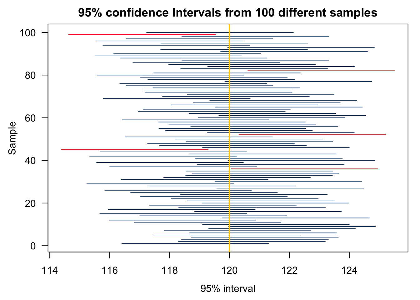
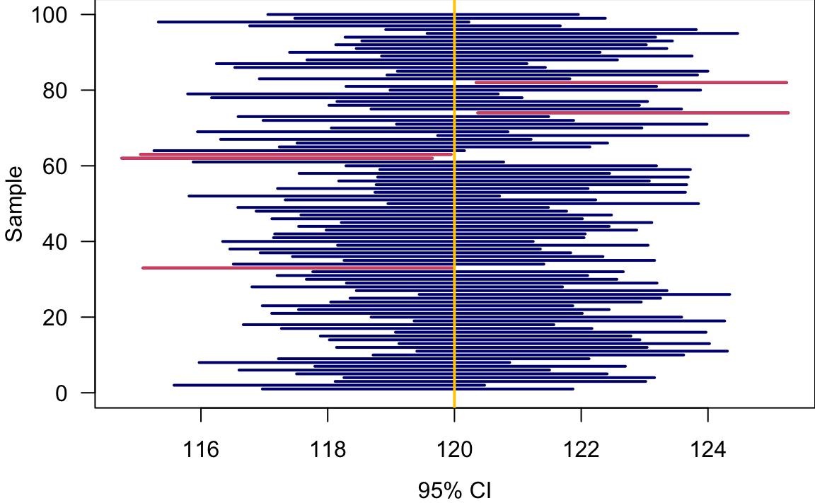
But still what does “95% confident” really mean? This means if we were able to collect our data many times and build the corresponding CIs, we would expect that about 95% of those intervals would contain the true population parameter, which, in this case, is the mean systolic blood pressure.

Remember that $\bar{x}$ varies from sample to sample, so does its corresponding CI because the CI is a function of $\bar{X}$ given $n$ and $\sigma$. This idea is shown in Figure 14.5. Here we do a simulation assuming $\mu$ is known at 120, and $\sigma =5$. Also, assume we were able to repeatedly collect our sample of the same size $n=16$. Here 100 data sets are generated, and for each data set, the sample mean and its corresponding 95% CI are computed. Since the confidence level is 95%, 95% of those intervals would contain the true population parameter, 120 in this example. The 36th, 45th, 52nd, 82nd, and 99th data sets have the interval not capturing the true parameter.

Figure 14.5: Illustration of 100 95% confidence intervals.

Important

Please keep the following ideas in mind.

1. A 95% CI does not mean that if 100 data sets are collected, there will be exactly 95 intervals capturing $\mu$. It is a long-term sampling idea.

2. We never know with certainty that 95% of the intervals, or any single interval for that matter, contains the true population parameter because again we never know what the true value of the parameter is.

3. In reality, we usually have only one data set, and we are not able to collect more data. We have no idea of whether our 95% confidence interval capture the unknown parameter or not. We are only “95% confident”.

The procedure of generating 100 confidence intervals for $\mu$ when $\sigma$ is known is shown in the algorithm below.

Algorithm

Algorithm

1. Generate 100 sampled data of size $n$: $(x_1^1,x_2^1,\dots ,x_n^1),\dots (x_1^{100},x_2^{100},\dots ,x_n^{100})$, where $x_i^m\sim N(\mu ,{\sigma }^2)$.

2. Obtain 100 sample means $({\bar{x}}^1,\dots ,{\bar{x}}^{100})$.

3. For each $m=1,2,\dots ,100$, compute the corresponding confidence interval $$({\bar{x}}^m-z_{\alpha /2}\frac{\sigma }{\sqrt{n}},{\bar{x}}^m+z_{\alpha /2}\frac{\sigma }{\sqrt{n}})$$

R Simulation Result

R Code

mu <- 120; sig <- 5 
al <- 0.05; M <- 100; n <- 16

set.seed(2024)
x_rep <- replicate(M, rnorm(n, mu, sig))
xbar_rep <- apply(x_rep, 2, mean)
E <- qnorm(p = 1 - al / 2) * sig / sqrt(n)
ci_lwr <- xbar_rep - E
ci_upr <- xbar_rep + E

plot(NULL, xlim = range(c(ci_lwr, ci_upr)), ylim = c(0, M), 
     xlab = "95% CI", ylab = "Sample", las = 1)
mu_out <- (mu < ci_lwr | mu > ci_upr)
segments(x0 = ci_lwr, y0 = 1:M, x1 = ci_upr, col = "navy", lwd = 2)
segments(x0 = ci_lwr[mu_out], y0 = (1:M)[mu_out], x1 = ci_upr[mu_out], 
         col = 2, lwd = 2)
abline(v = mu, col = "#FFCC00", lwd = 2)

Python Simulation Result

# (114.22947438766174, 125.53817008417028)
# (0.0, 100.0)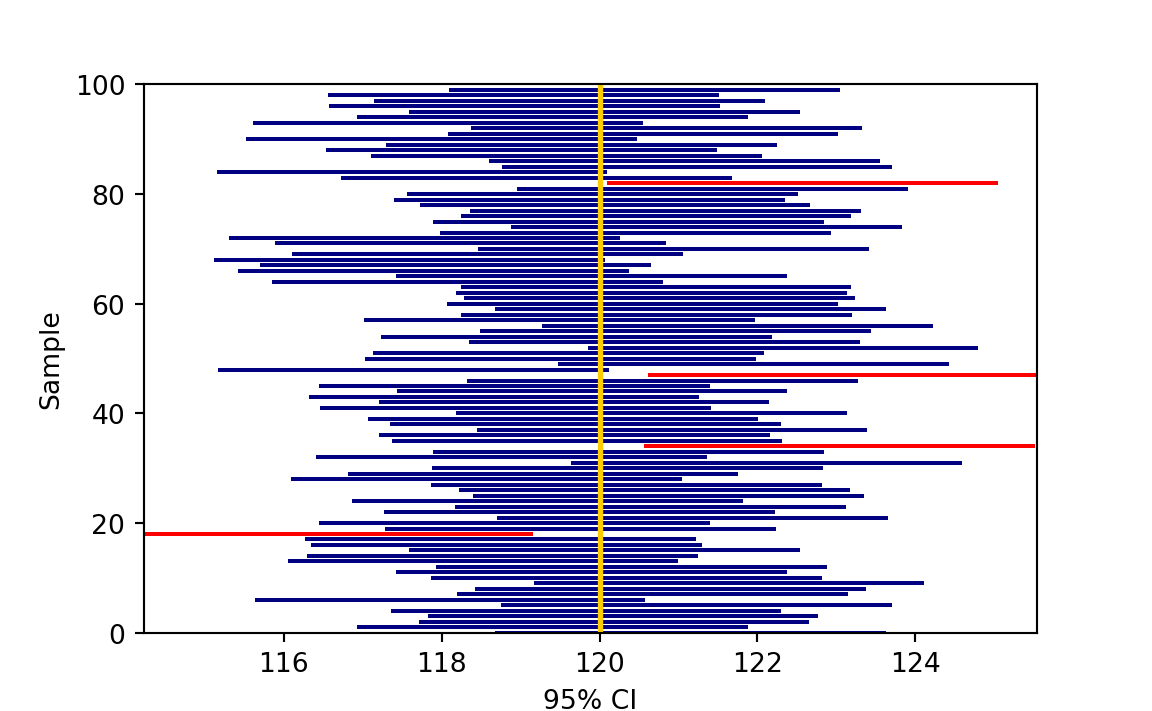

Python Code

mu = 120
sig = 5
al = 0.05
M = 100
n = 16

np.random.seed(2024)
x_rep = np.random.normal(loc=mu, scale=sig, size=(M, n))
xbar_rep = np.mean(x_rep, axis=1)
E = norm.ppf(1 - alpha / 2) * sig / np.sqrt(n)
ci_lwr = xbar_rep - E
ci_upr = xbar_rep + E

for i in range(M):
    col = 'red' if mu < ci_lwr[i] or mu > ci_upr[i] else 'navy'
    plt.plot([ci_lwr[i], ci_upr[i]], [i, i], color=col, lw=1.5)
plt.xlim([min(ci_lwr), max(ci_upr)])
plt.ylim([0, M])
plt.xlabel("95% CI")
plt.ylabel("Sample")
plt.axvline(mu, color="#FFCC00", lw=2)
plt.show()

14.3.1 Reducing margin of error and determining sample size*

We learn that the margin of error is $E=z_{\alpha /2}\frac{\sigma }{\sqrt{n}}$. Of course we prefer small margin of error for more estimation accuracy and precision. From its formula, we can see that there are three ways to reduce the margin of error:

• Reduce $\sigma$
• Increase $n$
• Reduce $z_{\alpha /2}$

However, given a confidence level $1-\alpha$ and known $\sigma$, we can reduce the margin of error only by increasing sample size $n$. Due to high sampling costs, we like to find the minimum sample size needed to get a desired margin of error.

What we can do is to rewrite the margin of error, and represent $n$ as a function of $E$, $\alpha$, and $\sigma$. Once all three are given, we know the how large the sample size is.

$E=z_{\alpha /2}\frac{\sigma }{\sqrt{n}}⟺\frac{1}{\sqrt{n}}=\frac{E}{z_{\alpha /2}\sigma }⟺\sqrt{n}=\frac{z_{\alpha /2}\sigma }{E}⟺n={\left(\frac{z_{\alpha /2}\sigma }{E}\right)}^2$

Clearly, to get the desired margin of error, say $E_d$ the sample size should be at least ${\left(\frac{z_{\alpha /2}\sigma }{E_d}\right)}^2$ because $E$ and $n$ inversely proportional to each other.

---

Example

State tax advisory board wants to estimate the mean household income with a margin of error of $1,000 with 99% confidence level. Assume that the population standard deviation is $10,000. How many households they need to sample?

• $E=1000$, $\alpha =0.01$ and $z_{0.005}=2.58$, $\sigma =10000$

• $n={\left(\frac{z_{\alpha /2}\sigma }{E}\right)}^2={\left(\frac{(2.58)(10000)}{1000}\right)}^2=656.7$

• They need sample size 657.

14.4 Confidence Intervals for $\mu$ When $\sigma$ is Unknown

We complete the discussion of confidence intervals for $\mu$ when $\sigma$ is known. Do you see anything unreasonable? Do you think that assuming ${\sigma }^2$ is known is reasonable? In fact, the population variance is calculated as ${\sigma }^2=\frac{\sum _{i=1}^N(x_i-\mu {)}^2}{N}$, where $N$ is the population size. The formula involves $\mu$, the unknown parameter we’d like to estimate. It’s rare that we don’t know $\mu$ but know $\sigma$. What do we do if $\sigma$ is unknown?

When $\sigma$ is unknown to us, we cannot use normal distribution anymore. Instead, we use the Student’s t distribution (or $t$-distribution) to construct a confidence interval for $\mu$ when $\sigma$ is unknown. To construct these confidence intervals we still need

• A random sample
• A population that is normally distributed and/or $n>30$.

The confidence interval when $\sigma$ is known includes $\sigma$ in the formula. When $\sigma$ is unknown, we cannot use the formula and need to find $\sigma$’s surrogate.

What is a natural estimator for the unknown $\sigma$?

When $\sigma$ is unknown, we use the sample standard deviation, $S=\sqrt{\frac{\sum _{i=1}^n(X_i-\bar{X}{)}^2}{n-1}}$, instead when constructing the CI.

---

Student’s t Distribution

If the population is normally distributed or $n>30$, we know $\bar{X}$ is exactly or approximately $N(\mu ,\frac{{\sigma }^2}{n})$. Therefore $Z=\frac{\bar{X}-\mu }{\sigma /\sqrt{n}}\sim N(0,1)$. Now if $\sigma$ is replaced with its surrogate $S$, then the new random variable say $T$ will be student’s t distributed with the degrees of freedom (df) $n-1$:

$$T=\frac{\bar{X}-\mu }{S/\sqrt{n}}\sim t_{n-1}$$

Here the degrees of freedom is the parameter of the student’s t distribution.

Properties

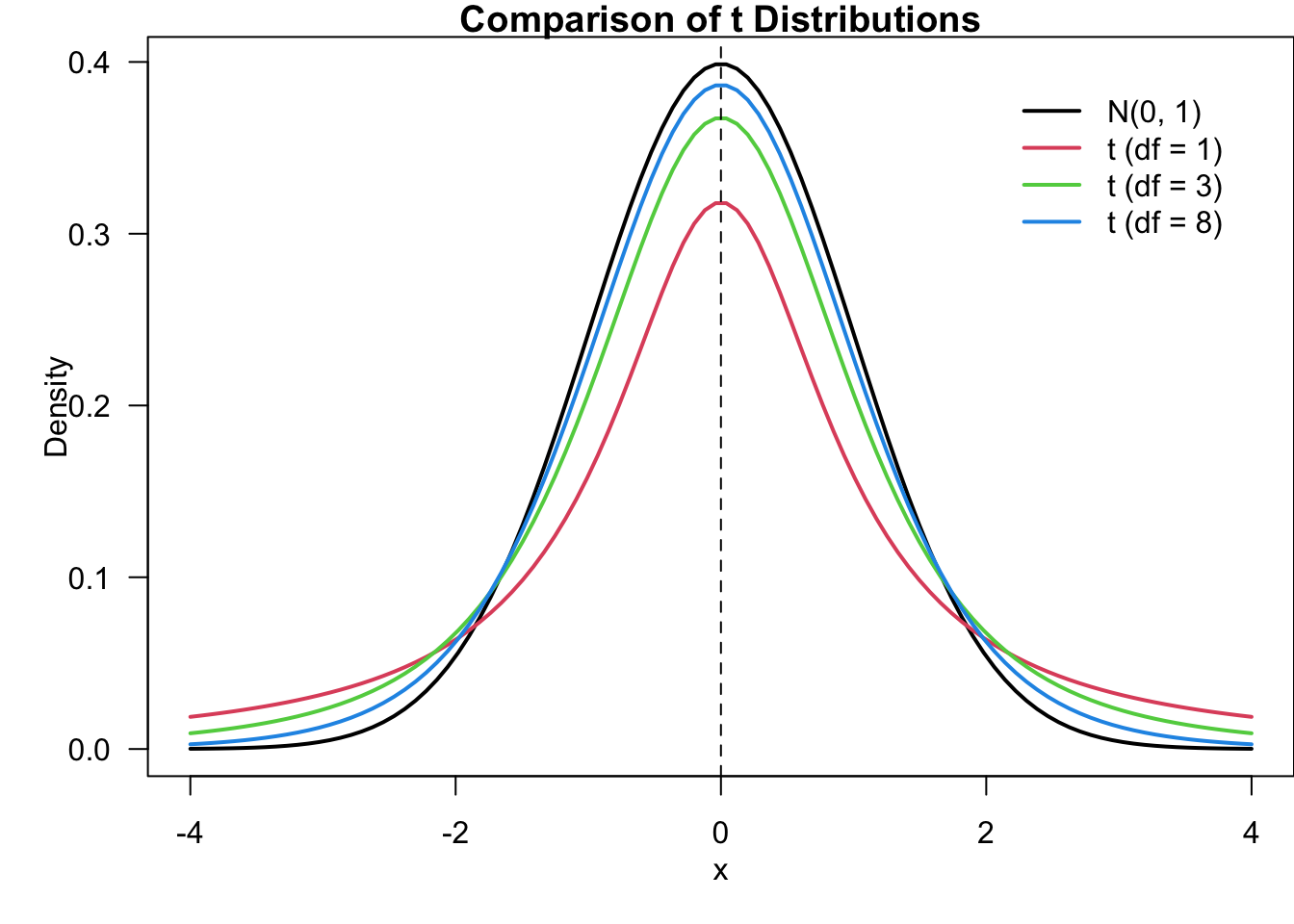
The student’s t distribution, as shown in Figure 14.6, looks pretty similar to the standard normal distribution, but they are different. Some of the properties of the student’s t distribution are listed below.

• For any degrees of freedom, the student’s t distribution is symmetric about the mean 0 and bell-shaped like $N(0,1)$.

• For any degrees of freedom, the student’s t distribution has more variability than $N(0,1)$, meaning that the distribution has heavier tails and lower peak.

• The the student’s t distribution has less variability for larger degrees of freedom (sample size).

• As $n\to \mathrm{\infty }$ $(df\to \mathrm{\infty })$, the student’s t distribution approaches $N(0,1)$.

Figure 14.6: Student t distributions with various degrees of freedom.

Critical Values of $t_{\alpha /2,n-1}$

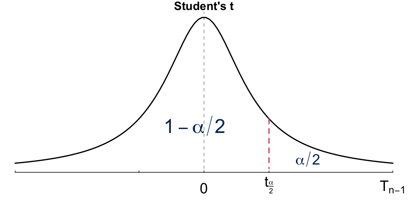
In the CI formula with known $\sigma$, we use the critical value $z_{\alpha /2}$, the standard normal value so that $P(Z>z_{\alpha /2})=\alpha /2$. When $\sigma$ is unknown, we use $t_{\alpha /2,n-1}$ as the critical value, instead of $z_{\alpha /2}$. Notice that the standard normal has nothing to do with $\mu$ and $\sigma$ of a general $N(\mu ,{\sigma }^2)$ distribution. ¹ Therefore no parameter is attached to $z_{\alpha /2}$. However, the $t$ critical value $t_{\alpha /2,n-1}$ changes with the degrees of freedom $n-1$. With the same logic, the critical value $t_{\alpha /2,n-1}$ is a Student’s t value with degrees of freedom $n-1$ so that $P(T_{n-1}>t_{\alpha /2,n-1})=\alpha /2$ as shown in Figure 14.7.

Figure 14.7: Illustration of critical value for Student t distribution.

With the same $\alpha$, is $t_{\alpha ,n-1}$ or $z_{\alpha }$ larger?

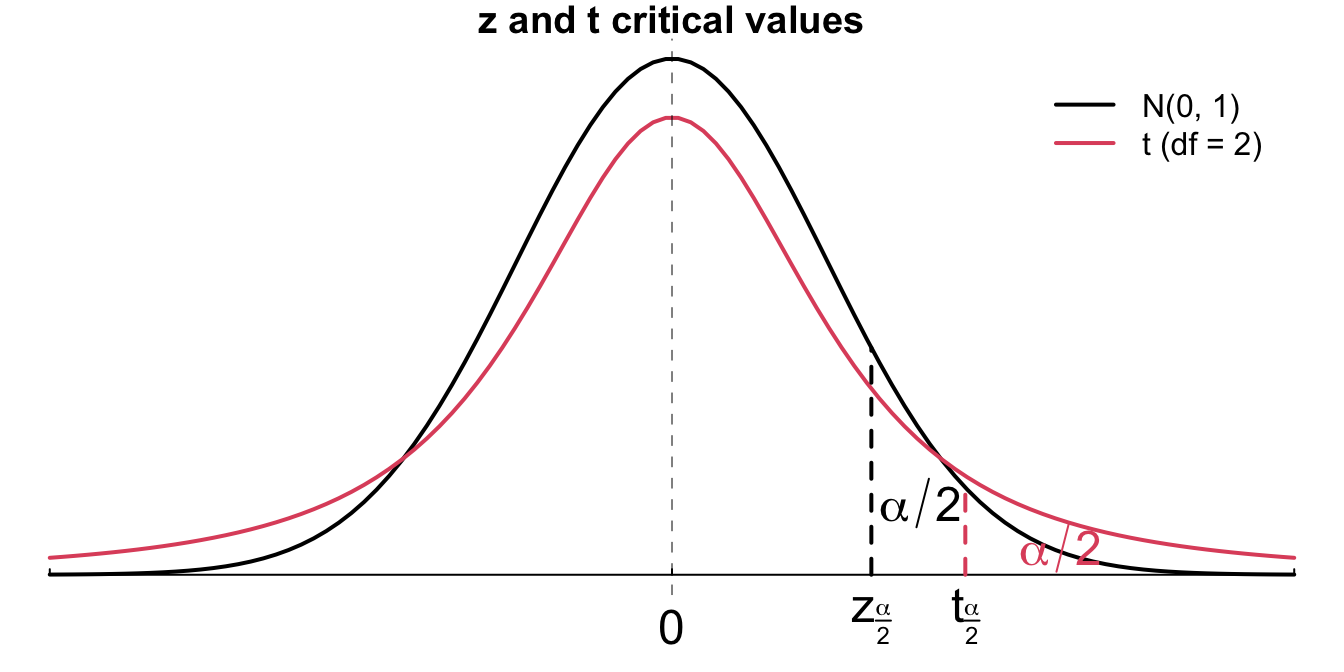
You should be able to answer this question based on the fact that for any degrees of freedom, the student’s t distribution has more variability than $N(0,1)$, or heavier tails. The heavier tail forces $t_{\alpha /2,n-1}$ to be more extreme than $z_{\alpha /2}$. Figure 14.8 illustrates this fact. The red $t_{df=2}$ distribution has heavier tails than the black standard normal distribution.

Figure 14.8: z and t critical values.

The table below shows $z$ and $t$ critical values at confidence level 90%, 95% and 99%. The $t$ values are getting closer to the $z$ values as the degree of freedom increases. When the degree of freedom goes to infinity, the $t$ values converge to $z$ values.

Level	t df = 5	t df = 15	t df = 30	t df = 1000	t df = inf	z
90%	2.02	1.75	1.70	1.65	1.64	1.64
95%	2.57	2.13	2.04	1.96	1.96	1.96
99%	4.03	2.95	2.75	2.58	2.58	2.58

---

$(1-\alpha )100\mathrm{\%}$ Confidence Intervals for $\mu$ When $\sigma$ is Unknown

We have been equipped with everything we need for constructing $(1-\alpha )100\mathrm{\%}$ confidence interval for $\mu$ when $\sigma$ is unknown. The interval is $$(\bar{x}-t_{\alpha /2,n-1}\frac{s}{\sqrt{n}},\bar{x}+t_{\alpha /2,n-1}\frac{s}{\sqrt{n}})$$

The interval form is the same as before. We have the sample mean plus and minus the margin of error. Comparing to the interval with known $\sigma$, the difference is that $z_{\alpha /2}$ is replaced with $t_{\alpha /2,n-1}$, and $\sigma$ is replaced with $s$.

Given the same confidence level $1-\alpha$, $t_{\alpha /2,n-1}>z_{\alpha /2}$, leading to a wider interval if $s$ is not too smaller than the true $\sigma$. The intuition is that we are more uncertain when doing inference about $\mu$ because we don’t have information about both $\mu$ and $\sigma$, and replacing $\sigma$ with $s$ adds additional uncertainty.

R

Back to the systolic blood pressure (SBP) example. We have $n=16$ and $\bar{x}=121.5$. Estimate the mean SBP with a 95% confidence interval with unknown $\sigma$ and $s=5$. The code for the $t$ interval is pretty similar to the $z$ interval. The main difference is that we are gonna use qt() to find a quantile or critical value from the Student’s t distribution. In the function, the first argument is still the given probability, then we must specify the degrees of freedom, otherwise R cannot determine which $t$-distribution is being considered, and will render an error message.

alpha <- 0.05
n <- 16
x_bar <- 121.5
s <- 5  ## sigma is unknown and s = 5

## t-critical value
(cri_t <- qt(p = alpha / 2, df = n - 1, lower.tail = FALSE)) 
# [1] 2.13

## margin of error
(m_t <- cri_t * (s / sqrt(n)))  
# [1] 2.66

## 95% CI for mu when sigma is unknown
x_bar + c(-1, 1) * m_t  
# [1] 119 124

Python

Back to the systolic blood pressure (SBP) example. We have $n=16$ and $\bar{x}=121.5$. Estimate the mean SBP with a 95% confidence interval with unknown $\sigma$ and $s=5$. The code for the $t$ interval is pretty similar to the $z$ interval. The main difference is that we are gonna use t.ppf() (or t.isf()) to find a quantile or critical value from the Student’s t distribution. In the function, the first argument is still the given probability, then we must specify the degrees of freedom, otherwise Python cannot determine which $t$-distribution is being considered, and will render an error message.

alpha = 0.05
n = 16
x_bar = 121.5
s = 5  # Sample standard deviation (sigma unknown)

from scipy.stats import t
## t-critical value
cri_t = t.ppf(1 - alpha/2, df=n-1)
cri_t
# 2.131449545559323

## margin of error
m_t = cri_t * (s / np.sqrt(n))
m_t
# 2.664311931949154

## 95% CI for mu when sigma is unknown
x_bar + np.array([-1, 1]) * m_t  
# array([118.83568807, 124.16431193])

$z_{0.025}=1.96<t_{0.025,15}=2.13$. The interval is wider with $s=5$.

14.5 Summary

To conclude this chapter, a table that summarizes the confidence interval for $\mu$ is provided.

	Numerical Data, $\sigma$ known	Numerical Data, $\sigma$ unknown
Parameter of Interest	Population Mean $\mu$	Population Mean $\mu$
Confidence Interval	$\overline{x}\pm z_{\alpha /2}\frac{\sigma }{\sqrt{n}}$	$\overline{x}\pm t_{\alpha /2,n-1}\frac{s}{\sqrt{n}}$

Remember to check if the population is normally distributed and/or $n>30$. What if the population is not normal and $n\le 30$? We could use a simulation-based approach, for example bootstrapping discussed in Chapter 15.

14.6 Exercises

1. Here are summary statistics for randomly selected weights of newborn boys: $n=207$, $\overline{x}=30.2$hg (1hg = 100 grams), $s=7.3$hg.

   1. Compute a 95% confidence interval for $\mu$, the mean weight of newborn boys.
   2. Is the result in (a) very different from the 95% confidence interval if $\sigma =7.3$?

2. A 95% confidence interval for a population mean $\mu$ is given as (18.635, 21.125). This confidence interval is based on a simple random sample of 32 observations. Calculate the sample mean and standard deviation. Assume that all conditions necessary for inference are satisfied. Use the t-distribution in any calculations.

3. A market researcher wants to evaluate car insurance savings at a competing company. Based on past studies he is assuming that the standard deviation of savings is $95. He wants to collect data such that he can get a margin of error of no more than $12 at a 95% confidence level. How large of a sample should he collect?

4. The 95% confidence interval for the mean rent of one bedroom apartments in Chicago was calculated as ($2400, $3200).

   1. Interpret the meaning of the 95% interval.
   2. Find the sample mean rent from the interval.

---

1. The standard normal random variable $Z\sim N(0,1)$ is a pivotal quantity (or pivot) because it is independent of parameters $\mu$ and $\sigma$.