
17 Comparing Two Population Means
17.1 Introduction
Why Compare Two Populations?
We’ve discussed estimation (Chapter 14) and hypothesis testing (Chapter 16) for one single population mean \(\mu.\) The methods we learned can only be used for one sample or population. However, quite often we are faced with a comparison of parameters from different populations. For example,
Comparing the mean annual income for Male and Female groups.
Testing if a diet used for losing weight is effective from Placebo samples and New Diet samples.
If these two samples are drawn from two target populations with means, \(\mu_1\) and \(\mu_2\) respectively, the testing problem can be formulated as \[\begin{align} &H_0: \mu_1 = \mu_2 \\ &H_1: \mu_1 > \mu_2 \end{align}\]
where \(\mu_1\) for example is the male mean annual income and \(\mu_2\) is the female mean annual income Or \(\mu_1\) is the mean weight loss from the New Diet group, and \(\mu_2\) is the mean weight loss from the Placebo group.
To compare two means, we need two samples, one for one mean. But the two samples may be dependent or independent, and the methods for comparing two means depend on whether the two samples are dependent or not. So let’s see what dependent and independent samples are.
Dependent and Independent Samples
The two samples used to compare two population means can be independent or dependent.
Two samples are dependent or matched pairs if the sample values are matched, where the matching is based on some inherent relationship. For example,
Height data of fathers and daughters, where the height of each dad is matched with the height of his daughter. Clearly, father and daughter share the same life style, genes, and other factors that affect both father and daughter’s height. So the taller the father is, the taller the daughter tends to be. Their heights are positively correlated. In the two sample data sets, the first father height in the father’s sample is paired with the first daughter height in the daughter’s sample. Same for the second pair, third pair, and so on.
Weights of subjects measure before and after some diet treatment, where the subjects are the same both before and after treatments. In this example, we again have two samples. The two samples are dependent because the subjects in the two samples are identical. Your weight today is of course related to your weight last week, right? In the two sample data sets, the first weight in the sample before diet treatment is paired with the first weight in the sample after treatment. The two sample values belong to the same person. Same for the second pair, third pair, and so on.

Dependent Samples (Matched Pairs)
From the two examples, we learn that subject 1 may refer to
- the first matched pair (dad-daughter)
- the same person with two measurements (before and after treatment)
If we have data with only one variable, in R the data is usually saved as a vector. When we have two samples, the two samples can be saved as a vector separately, or saved as a data matrix with the two samples combined by columns like the table below. Each row is for one matched pair, or the same subject. One column is for one sample data. Note that since every subject in dependent samples is paired, the two samples are of the same size \(n\).
| Subject | (Dad) Before | (Daughter) After |
|---|---|---|
| 1 | \(x_{b1}\) | \(x_{a1}\) |
| 2 | \(x_{b2}\) | \(x_{a2}\) |
| 3 | \(x_{b3}\) | \(x_{a3}\) |
| \(\vdots\) | \(\vdots\) | \(\vdots\) |
| \(n\) | \(x_{bn}\) | \(x_{an}\) |
Independent Samples
Two samples are independent if the sample values from one population are not related to the sample values from the other. For example,
- Salary samples of men and women, where the two samples are drawn independently from the male and female groups.

We may want to compare the mean salary level of male and female. What we can do is to collect two samples independently, one for each group, from their own population. Any subject in the male group has nothing to do with any subject in the female group, and any subject in the male group cannot be paired with any subject in the female group in any way.
The independent samples can be summarized as the table below. Notice that the two samples can have different sample sizes, \(n_1\) and \(n_2\) for example. Because the subjects in the two samples are not paired, we can collect salary data from 50 males and 65 females. In the data table, \(x_{14}\) means the 4th subject measurement in the first group, and \(x_{23}\) means the 3rd subject measurement in the second group. In general, \(x_{ij}\) is the \(j\)-th measurement in the \(i\)-th group.
| Subject of Group 1 (Male) | Measurement of Group 1 | Subject of Group 2 (Female) | Measurement of Group 2 |
|---|---|---|---|
| 1 | \(x_{11}\) | 1 | \(x_{21}\) |
| 2 | \(x_{12}\) | 2 | \(x_{22}\) |
| 3 | \(x_{13}\) | 3 | \(x_{23}\) |
| \(\vdots\) | \(\vdots\) | \(\vdots\) | \(\vdots\) |
| \(n_1\) | \(x_{1n_1}\) | \(\vdots\) | \(\vdots\) |
| \(n_2\) | \(x_{2n_2}\) |
Inference from Two Samples
The statistical methods are different for these two types of samples. The good news is the concepts of confidence intervals and hypothesis testing for one population can be applied to two-population cases.
Let’s quickly review the confidence interval and test statistic in the one-sample case.
\(\text{CI = point estimate} \pm \text{margin of error (E)}\)
- e.g., \(\overline{x} \pm t_{\alpha/2, n-1} \frac{s}{\sqrt{n}}\)
Margin of error = critical value \(\times\) standard error of the point estimator
The 6 testing steps are the same, and both critical value and \(p\)-value method can be applied too.
- e.g., \(t_{test} = \frac{\overline{x} - \mu_0}{s/\sqrt{n}}\)
17.2 Inferences About Two Means: Dependent Samples (Matched Pairs)
In this section we talk about the inference methods for comparing two population means when the samples are dependent.
Hypothesis Testing for Dependent Samples
To analyze a paired data set, we can simply analyze the differences!
Suppose we would like to learn if the population means \(\mu_1\) and \(\mu_2\) are different. We can conduct a test like \[\begin{align} &H_0: \mu_1 = \mu_2 \\ &H_1: \mu_1 \ne \mu_2 \end{align}\]
The null hypothesis can also be written as \(H_0: \mu_1 - \mu_2 = 0\). We don’t really want to know the value of \(\mu_1\) and/or \(\mu_2\), and we just care about if they are equal, or their difference is zero. Therefore, if we let \(\mu_d\) be the difference \(\mu_1 - \mu_2\), we can write our hypothesis as \[\begin{align} &H_0: \mu_d = 0 \\ &H_1: \mu_d \ne 0 \end{align}\]
or more generally for any types of test,
\[\begin{align} & H_0: \mu_1 - \mu_2 = 0 \iff \mu_d = 0 \\ & H_1: \mu_1 - \mu_2 > 0 \iff \mu_d > 0 \\ & H_1: \mu_1 - \mu_2 < 0 \iff \mu_d < 0 \\ & H_1: \mu_1 - \mu_2 \ne 0 \iff \mu_d \ne 0 \end{align}\]
For dependent samples, we just transform the two samples into one difference sample by taking the difference between paired measurements. We use the difference sample to do the inference about the mean difference. The data table below illustrate the idea. We create a new difference sample data \((d_1, d_2, \dots, d_n)\) where the \(i\)-th sample difference is \(x_{1i} - x_{2i}\), the difference between the \(i\)-th measurement in the first sample and the \(i\)-th measurement in the second sample.
| Subject | \(x_1\) | \(x_2\) | Difference \(d = x_1 - x_2\) |
|---|---|---|---|
| 1 | \(x_{11}\) | \(x_{21}\) | \(\color{red}{d_1}\) |
| 2 | \(x_{12}\) | \(x_{22}\) | \(\color{red}{d_2}\) |
| 3 | \(x_{13}\) | \(x_{23}\) | \(\color{red}{d_3}\) |
| \(\vdots\) | \(\vdots\) | \(\vdots\) | \(\color{red}{\vdots}\) |
| \(n\) | \(x_{1n}\) | \(x_{2n}\) | \(\color{red}{d_n}\) |
The sample \((d_1, d_2, \dots, d_n)\) is used to estimate the mean difference \(\mu_d = \mu_1 - \mu_2\). So what is our point estimate of \(\mu_d\)? The point estimate is the sample average of \((d_1, d_2, \dots, d_n)\) which is \(\overline{d}\). Actually, the point estimate is equal to \(\overline{x}_1 - \overline{x}_2\), the estimate for \(\mu_1 - \mu_2\).
Inference for Paired Data
Here are the requirements for the inference for paired data. The sample differences \(\color{blue}{d_i}\)s form a random sample, and they are from a normal distribution and/or the sample size \(n > 30\). Remember that when analyzing paired data, we focus on the difference of measurements, and this \(d_i\) sample becomes our new one single sample for inference about one single population parameter, the mean difference \(\mu_d\).
With this, the inference for paired data follows the same procedure as the one-sample \(t\)-test! Therefore, the test statistic is \[\color{blue}{t_{test} = \frac{\overline{d}-\mu_d}{s_d/\sqrt{n}}} = \frac{\overline{d}-0}{s_d/\sqrt{n}} \sim T_{n-1}\] under \(H_0\) where \(\overline{d}\) and \(s_d\) are the mean and standard deviation of the difference samples \((d_1, d_2, \dots, d_n)\).
The critical value is either \(t_{\alpha, n-1}\) or \(t_{\alpha/2, n-1}\) depending on if it is a one-tailed or two-tailed test. Below is a table summarizing information necessary to make inferences about paired data.
| Paired \(t\)-test | Test Statistic | Confidence Interval for \(\mu_d = \mu_1 - \mu_2\) |
|---|---|---|
| \(\sigma_d\) is unknown | \(\large t_{test} = \frac{\overline{d}}{s_d/\sqrt{n}}\) | \(\large \overline{d} \pm t_{\alpha/2, n-1} \frac{s_d}{\sqrt{n}}\) |
The test for matched pairs is called a paired \(t\)-test.
Example
Consider a capsule used to reduce blood pressure (BP) for individuals with hypertension. A sample of 10 individuals with hypertension takes the medicine for 4 weeks. The BP measurements before and after taking the medicine are shown in the table below. Does the data provide sufficient evidence that the treatment is effective in reducing BP?
| Subject | Before \((x_b)\) | After \((x_a)\) | Difference \(d = x_b - x_a\) |
|---|---|---|---|
| 1 | 143 | 124 | 19 |
| 2 | 153 | 129 | 24 |
| 3 | 142 | 131 | 11 |
| 4 | 139 | 145 | -6 |
| 5 | 172 | 152 | 20 |
| 6 | 176 | 150 | 26 |
| 7 | 155 | 125 | 30 |
| 8 | 149 | 142 | 7 |
| 9 | 140 | 145 | -5 |
| 10 | 169 | 160 | 9 |
Given the data \(x_b\) and \(x_a\), we first take the difference and create the new data \(d = x_b - x_a\) for each subject.
Step 1
- If we let \(\mu_1 =\) Mean Before, \(\mu_2 =\) Mean After, and \(\mu_d = \mu_1 - \mu_2\), then the hypothesis is \(\begin{align} &H_0: \mu_1 = \mu_2 \iff \mu_d = 0\\ &H_1: \mu_1 > \mu_2 \iff \mu_d > 0 \end{align}\) The key is that “the treatment is effective in reducing BP” means the mean BP after taking the medicine is lower than that before, so \(\mu_1 > \mu_2\).
Step 2
- \(\alpha = 0.05\)
Step 3
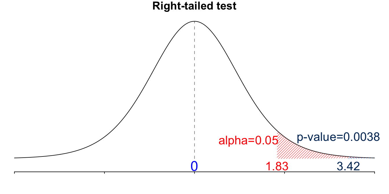
For the \(d\) sample, \(\overline{d} = 13.5\), \(s_d= 12.48\). \(t_{test} = \frac{\overline{d}}{s_d/\sqrt{n}} = \frac{13.5}{12.48/\sqrt{10}} = 3.42.\)
Step 4-c
- This is a right-tailed test. \(t_{\alpha, n-1} = t_{0.05, 9} = 1.833\).
Step 5-c
- We reject \(H_0\) if \(\small t_{test} > t_{\alpha, n-1}\). Since \(\small t_{test} = 3.42 > 1.833 = t_{\alpha, n-1}\), we reject \(H_0\).
Step 6
- There is sufficient evidence to support the claim that the drug is effective in reducing blood pressure.
The 95% CI for \(\mu_d = \mu_1 - \mu_2\) is \[\begin{align}\overline{d} \pm t_{\alpha/2, df} \frac{s_d}{\sqrt{n}} &= 13.5 \pm t_{0.025, 9}\frac{12.48}{\sqrt{10}}\\ &= 13.5 \pm 8.927 \\ &= (4.573, 22.427).\end{align}\]
We are 95% confident that the mean difference in blood pressure is between 4.57 and 22.43. Since the interval does NOT include 0, it leads to the same conclusion as rejection of \(H_0\).
Below is the same data as in the previous hypertension example. We load the R data pair_data.RDS into the R session using the load() function.
# Load the data set
load("../introstatsbook/data/pair_data.RDS")
pair_data
before after
1 143 124
2 153 129
3 142 131
4 139 145
5 172 152
6 176 150
7 155 125
8 149 142
9 140 145
10 169 160## Create the difference data d
(d <- pair_data$before - pair_data$after) [1] 19 24 11 -6 20 26 30 7 -5 9## sample mean of d
(d_bar <- mean(d))[1] 13.5## sample standard deviation of d
(s_d <- sd(d))[1] 12.48332[1] 3.419823[1] 1.833113[1] 0.003815036Below is an example of how to calculate the confidence interval for the change in blood pressure.
## 95% confidence interval for the mean difference of the paired data
d_bar + c(-1, 1) * qt(p = 0.975, df = length(d) - 1) * (s_d / sqrt(length(d)))
[1] 4.569969 22.430031We can see that performing these calculations in R leads us to the same conclusions we previously made. In fact, the R function t.test() does Student’s t-test for us, either one sample or two samples. To do the two sample paired \(t\) test, we provides the two samples in the argument x and y. The alternative argument is either “two.sided”, “less” or “greater”. We have \(H_1: \mu_1 > \mu_2\) or \(\mu_d > 0\), so we use “greater”. The argument \mu is the difference in means in \(H_0\), which is zero in our case. Finally, the paired argument should be set as TRUE in order to do the paired \(t\) test.
## t.test() function
t.test(x = pair_data$before, y = pair_data$after,
       alternative = "greater", mu = 0, paired = TRUE)
    Paired t-test

data:  pair_data$before and pair_data$after
t = 3.4198, df = 9, p-value = 0.003815
alternative hypothesis: true mean difference is greater than 0
95 percent confidence interval:
 6.263653      Inf
sample estimates:
mean difference
           13.5
Note that we get the same test statistic and p-value, as well as the test conclusion. However, the one-sided 95% confidence interval shown in the output is not what we want! We may have a one-sided or two-sided test, but we should always use the two-sided confidence interval. When you use the t.test() function to do a one-sided test as we do here, please do not use the confidence interval in the output.
import numpy as np
from scipy.stats import ttest_rel, t, norm
import pandas as pd
Below is the same data as in the previous hypertension example. We load the csv file pair_data.csv into the Python session using the pd.read_csv() function.
pair_data = pd.read_csv('./data/pair_data.csv')
pair_data
before after
0 143 124
1 153 129
2 142 131
3 139 145
4 172 152
5 176 150
6 155 125
7 149 142
8 140 145
9 169 160# Create the difference data 'd'
d = pair_data['before'] - pair_data['after']
d0 19
1 24
2 11
3 -6
4 20
5 26
6 30
7 7
8 -5
9 9
dtype: int64# Sample mean of 'd'
d_bar = np.mean(d)
d_bar13.5# Sample standard deviation of 'd'
s_d = np.std(d, ddof=1)
s_d12.48332220738267# T-test statistic
t_test = d_bar / (s_d / np.sqrt(len(d)))
t_test3.4198226804580676# T critical value (one-tailed, 95% confidence level)
t.ppf(0.95, df=len(d)-1)1.8331129326536335# P-value
t.sf(t_test, df=len(d)-1)0.0038150362846879134Below is an example of how to calculate the confidence interval for the change in blood pressure.
# 95% confidence interval for the mean difference
d_bar + pd.Series([-1, 1]) * t.ppf(0.975, df=len(d)-1) * (s_d / np.sqrt(len(d)))
0 4.569969
1 22.430031
dtype: float64We can see that performing these calculations in Python leads us to the same conclusions we previously made.
In fact, the Python function ttest_rel() from the scipy.stats module does two sample paired t-test for us. The word rel means “related” because it calculates the t-test on TWO RELATED samples. To do the two sample paired \(t\) test, we provides the two samples in the first two arguments a and b. The alternative argument is either “two.sided”, “less” or “greater”. We have \(H_1: \mu_1 > \mu_2\) or \(\mu_d > 0\), so we use “greater”. The function only tests whether or not the mean difference is zero.
# T-test using scipy's built-in function
ttest_rel_res = ttest_rel(a=pair_data['before'], b=pair_data['after'],
                          alternative='greater')

ttest_rel_res.statistic3.419822680458067ttest_rel_res.df9ttest_rel_res.pvalue0.0038150362846879134ttest_rel_res.confidence_interval<bound method TtestResult.confidence_interval of TtestResult(statistic=3.419822680458067, pvalue=0.0038150362846879134, df=9)>Note that we get the same test statistic and p-value, as well as the test conclusion. The function does not print the confidence interval out though.
17.3 Inference About Two Means: Independent Samples
Compare Population Means: Independent Samples
Frequently we would like to compare two different groups. For example,
Whether stem cells can improve heart function. Here the two samples are patients with the stem cell treatment and the ones without the stem cell treatment.
The relationship between pregnant women’s smoking habits and newborns’ weights. Here the two samples are women who smoke and women who don’t.
Whether one variation of an exam is harder than another variation. In this case, the two samples are students having exam A and students taking exam B.


In those examples, the two samples are independent. In this section, we are going to learn how to compare their population means. For example, whether the mean score of exam A is higher than the mean score of exam B.
Testing for Independent Samples \((\sigma_1 \ne \sigma_2)\)
When we deal with two independent samples, we assume they are drawn from two independent populations which are assumed to be normally distributed in this chapter. We are interested in whether the two population means are equal or which is greater. But to do the inference, we need to take care of their standard deviation, \(\sigma_1\) and \(\sigma_2\). First we discuss the case when \(\sigma_1 \ne \sigma_2\).
The requirements of testing for independent samples with \(\sigma_1 \ne \sigma_2\) are
- The two samples are independent.
- Both samples are random samples.
- \(n_1 > 30\), \(n_2 > 30\) and/or both samples are from a normally distributed population. Large sample sizes are for the application of the central limit theorem. Note that both sample sizes should be large or at least greater than 30. If either one sample size is small, the inference methods discussed here are not valid.
We are interested in whether the two population means, \(\mu_1\) and \(\mu_2\), are equal or if one is larger than the other. Therefore, we have \[H_0: \mu_1 = \mu_2\]
This is equivalent to testing if their difference is zero, or \(H_0: \mu_1 - \mu_2 = 0\).
Sampling Distribution of \(\overline{X}_1 - \overline{X}_2\)
Again, to do the inference we start with the associated sampling distribution. If the two samples are from independent normally distributed populations or \(n_1 > 30\) and \(n_2 > 30\), then at least approximately
\[\small \overline{X}_1 \sim N\left(\mu_1, \frac{\sigma_1^2}{n_1} \right), \quad \overline{X}_2 \sim N\left(\mu_2, \frac{\sigma_2^2}{n_2} \right)\]
Because we use \(\overline{X}_1 - \overline{X}_2\) to estimate \(\mu_1 - \mu_2\), we need the sampling distribution of \(\overline{X}_1 - \overline{X}_2\). We won’t talk about the details, but it can be shown that \(\overline{X}_1 - \overline{X}_2\) has the sampling distribution \[\small \overline{X}_1 - \overline{X}_2 \sim N\left(\mu_1 - \mu_2, \frac{\sigma_1^2}{n_1} \color{red}{+} \color{black}{\frac{\sigma_2^2}{n_2}} \right). \] Before careful that the variance is the sum of the variance of \(\overline{X}_1\) and \(\overline{X}_2\), even the random variable is their difference. Please take MATH 4700 Introduction to Probability to learn more about the properties of normal distribution.
Therefore by standardization, we have a standard normal variable \[\small Z = \frac{(\overline{X}_1 - \overline{X}_2) - (\mu_1 - \mu_2)}{\sqrt{\frac{\sigma_1^2}{n_1} + \frac{\sigma_2^2}{n_2}}} \sim N(0, 1)\]
Test Statistic for Independent Samples \((\sigma_1 \ne \sigma_2)\)
With \(D_0\) being a hypothesized value, our testing problem could be one of the followings
\(\small \begin{align} &H_0: \mu_1 - \mu_2 \le D_0\\ &H_1: \mu_1 - \mu_2 > D_0 \end{align}\) (right-tailed)
\(\small \begin{align} &H_0: \mu_1 - \mu_2 \ge D_0\\ &H_1: \mu_1 - \mu_2 < D_0 \end{align}\) (left-tailed)
\(\small \begin{align} &H_0: \mu_1 - \mu_2 = D_0\\ &H_1: \mu_1 - \mu_2 \ne D_0 \end{align}\) (two-tailed)
Often, we care about of the two means are equal, so \(D_0\) is zero. But \(D_0\) could be any number that fits your research question. For example, you may wonder if mean weight of male is greater than the mean weight of female by 20 pounds. Then your \(H_1\) would be \(H_1: \mu_1 - \mu_2 > 20\) where \(\mu_1\) is the mean weight of male and \(\mu_2\) is the mean weight of female, and \(D_0\) is 20.
If \(\sigma_1\) and \(\sigma_2\) are known, with the \(\overline{x}_1\), \(\overline{x}_2\) calculated by our sample, and under the null hypothesis, the test statistic is the z-score from the sampling distribution which is \[z_{test} = \frac{(\overline{x}_1 - \overline{x}_2) - (\mu_1 - \mu_2)}{\sqrt{\frac{\sigma_1^2}{n_1} + \frac{\sigma_2^2}{n_2}}} = \frac{(\overline{x}_1 - \overline{x}_2) - \color{blue}{D_0}}{\sqrt{\frac{\sigma_1^2}{n_1} + \frac{\sigma_2^2}{n_2}}}.\]
Then we are pretty much done. We find \(z_{\alpha}\) or \(z_{\alpha/2}\) and follow our testing steps!
What if \(\sigma_1\) and \(\sigma_2\) are unknown? You should be able to sense the answer. The test statistic becomes \(t_{test}\):
\[t_{test} = \frac{(\overline{x}_1 - \overline{x}_2) - (\mu_1 - \mu_2)}{\sqrt{\frac{\color{red}{s_1^2}}{n_1} + \frac{\color{red}{s_2^2}}{n_2}}} = \frac{(\overline{x}_1 - \overline{x}_2) - \color{blue}{D_0}}{\sqrt{\frac{\color{red}{s_1^2}}{n_1} + \frac{\color{red}{s_2^2}}{n_2}}}. \]
We simply replace the unknown \(\sigma_1\) and \(\sigma_2\) with their corresponding sample estimate \(s_1\) and \(s_2\)! The critical value is either \(t_{\alpha, df}\) (one-tailed) or \(t_{\alpha/2, df}\) (two-tailed) with the degrees of freedom
\[df = \dfrac{(A+B)^2}{\dfrac{A^2}{n_1-1}+ \dfrac{B^2}{n_2-1}},\] where \(\small A = \dfrac{s_1^2}{n_1}\) and \(\small B = \dfrac{s_2^2}{n_2}\).
The degrees of freedom looks intimidating, but no worries you don’t need to memorize the formula, and we let the statistical software take care of it. To be conservative (tend to reject \(H_0\) less) if the \(df\) is not an integer, we round it down to the nearest integer, it does not matter much though.
Inference About Independent Samples \((\sigma_1 \ne \sigma_2)\)
Below is a table that summarizes ways to make inferences about independent samples when \((\sigma_1 \ne \sigma_2)\).
| \(\large \color{red}{\sigma_1 \ne \sigma_2}\) | Test Statistic | Confidence Interval for \(\mu_1 - \mu_2\) |
|---|---|---|
| known | \(\large z_{test} = \frac{(\overline{x}_1 - \overline{x}_2) - \color{blue}{D_0}}{\sqrt{\frac{\sigma_1^2}{n_1} + \frac{\sigma_2^2}{n_2}}}\) | \(\large (\overline{x}_1 - \overline{x}_2) \pm z_{\alpha/2} \sqrt{\frac{\sigma_1^2}{n_1} + \frac{\sigma_2^2}{n_2}}\) |
| unknown | \(\large t_{test} = \frac{(\overline{x}_1 - \overline{x}_2) - \color{blue}{D_0}}{\sqrt{\frac{\color{red}{s_1^2}}{n_1} + \frac{\color{red}{s_2^2}}{n_2}}}\) | \(\large (\overline{x}_1 - \overline{x}_2) \pm t_{\alpha/2, df} \sqrt{\frac{\color{red}{s_1^2}}{n_1} + \frac{\color{red}{s_2^2}}{n_2}}\) |
For unknown \(\sigma_1\) and \(\sigma_2\), we use \(\small df = \dfrac{(A+B)^2}{\dfrac{A^2}{n_1-1}+ \dfrac{B^2}{n_2-1}},\) where \(\small A = \dfrac{s_1^2}{n_1}\) and \(\small B = \dfrac{s_2^2}{n_2}\) to get the \(p\)-value, critical value and confidence interval. The unequal-variance t-test is called Welch’s t-test in the literature.
Example: Two-Sample t-Test
Does an over-sized tennis racket exert less stress/force on the elbow? The relevant sample statistics are shown below.
- Over-sized: \(n_1 = 33\), \(\overline{x}_1 = 25.2\), \(s_1 = 8.6\)
- Conventional: \(n_2 = 12\), \(\overline{x}_2 = 33.9\), \(s_2 = 17.4\)
The two populations are known to be nearly normal, and because of the large difference in the sample standard deviation suggests \(\sigma_1 \ne \sigma_2\). Please form a hypothesis test with \(\alpha = 0.05\), and construct a 95% CI for the mean difference of force on the elbow.

Step 1
- Let \(\mu_1\) be the mean force on the elbow for the over-size rackets, and \(\mu_2\) be the mean force for the conventional rackets. The we have a test \(\begin{align} &H_0: \mu_1 = \mu_2 \\ &H_1: \mu_1 < \mu_2 \end{align}\)
Step 2
- \(\alpha = 0.05\)
Step 3
- \(t_{test} = \frac{(\overline{x}_1 - \overline{x}_2) - (\mu_1-\mu_2)}{\sqrt{\frac{\color{red}{s_1^2}}{n_1} + \frac{\color{red}{s_2^2}}{n_2}}} = \frac{(25.2 - 33.9) - 0}{\sqrt{\frac{\color{red}{8.6^2}}{33} + \frac{\color{red}{17.4^2}}{12}}} = -1.66\)
- \(\small df = \dfrac{(A+B)^2}{\dfrac{A^2}{n_1-1}+ \dfrac{B^2}{n_2-1}},\) \(\small A = \dfrac{s_1^2}{n_1}\) and \(\small B = \dfrac{s_2^2}{n_2}\)
- \(\small A = \dfrac{8.6^2}{33}\), \(\small B = \dfrac{17.4^2}{12}\), \(\small df = \dfrac{(A+B)^2}{\dfrac{A^2}{33-1}+ \dfrac{B^2}{12-1}} = 13.01\)
Note
If the computed value of \(df\) is not an integer, always round down to the nearest integer.
Step 4-c
- Because it is a left-tailed test, the critical value is \(-t_{0.05, 13} = -1.771\).
Step 5-c
- We reject \(H_0\) if \(\small t_{test} < -t_{\alpha, df}\). \(\small t_{test} = -1.66 > -1.771 = -t_{\alpha, df}\), we fail to reject \(H_0\).
Step 6
- There is insufficient evidence to support the claim that the the oversized racket delivers less stress to the elbow.
The 95% CI for \(\mu_1 - \mu_2\) is
\[\begin{align}(\overline{x}_1 - \overline{x}_2) \pm t_{\alpha/2, df} \sqrt{\frac{\color{red}{s_1^2}}{n_1} + \frac{\color{red}{s_2^2}}{n_2}} &= (25.2 - 33.9) \pm t_{0.025,13}\sqrt{\frac{8.6^2}{33} + \frac{17.4^2}{12}}\\&= -8.7 \pm 11.32 = (-20.02, 2.62).\end{align}\]
We are 95% confident that the difference in the mean forces is between -20.02 and 2.62. Since the interval includes 0, it leads to the same conclusion as failing to reject \(H_0\).
Two-Sample t-Test in R
## Prepare needed variables
n1 = 33; x1_bar = 25.2; s1 = 8.6
n2 = 12; x2_bar = 33.9; s2 = 17.4
A <- s1^2 / n1; B <- s2^2 / n2
df <- (A + B)^2 / (A^2/(n1-1) + B^2/(n2-1))

## Use floor() function to round down to the nearest integer.
(df <- floor(df))
[1] 13## t_test
(t_test <- (x1_bar - x2_bar) / sqrt(s1^2/n1 + s2^2/n2))[1] -1.659894## t_cv
qt(p = 0.05, df = df)[1] -1.770933## p_value
pt(q = t_test, df = df)[1] 0.06042575# Prepare needed variables
n1 = 33; x1_bar = 25.2; s1 = 8.6
n2 = 12; x2_bar = 33.9; s2 = 17.4
A = s1**2 / n1; B = s2**2 / n2
df = (A + B)**2 / (A**2/(n1-1) + B**2/(n2-1))
# Round down to the nearest integer
df = np.floor(df)
df13.0# T-test statistic
t_test = (x1_bar - x2_bar) / np.sqrt(s1**2/n1 + s2**2/n2)
# T critical value
t.ppf(0.05, df=df)-1.7709333959867992# P-value
t.cdf(t_test, df=df)0.060425745501011804Testing for Independent Samples (\(\sigma_1 = \sigma_2 = \sigma\))
We’ve done the case that \(\sigma_1 \ne \sigma_2\). Now we are talking about the case when \(\sigma_1 = \sigma_2\). Because they are equal, the two \(\sigma\)s can be treated as one common \(\sigma\).
Sampling Distribution of \(\overline{X}_1 - \overline{X}_2\)
Again, we start with the sampling distribution of \(\overline{X}_1 - \overline{X}_2\) \[\overline{X}_1 - \overline{X}_2 \sim N\left(\mu_1 - \mu_2, \frac{\sigma_1^2}{n_1} + \frac{\sigma_2^2}{n_2} \right).\] If \(\sigma_1 = \sigma_2 = \sigma\), we can write \[\overline{X}_1 - \overline{X}_2 \sim N\left(\mu_1 - \mu_2, \sigma^2\left(\frac{1}{n_1} + \frac{1}{n_2} \right) \right).\] Therefore, \[ Z = \frac{(\overline{X}_1 - \overline{X}_2) - (\mu_1 - \mu_2)}{\sigma\sqrt{\frac{1}{n_1} + \frac{1}{n_2}}} \sim N(0, 1).\]
Test Statistic for Independent Samples \((\sigma_1 = \sigma_2 = \sigma)\)
Similar to the case that \(\sigma_1 = \sigma_2\), if \(\sigma_1\) and \(\sigma_2\) are known, the test statistic is the z-score of \(\overline{X}_1 - \overline{X}_2\) under \(H_0\): \[z_{test} = \frac{(\overline{x}_1 - \overline{x}_2) - (\mu_1 - \mu_2)}{\sigma\sqrt{\frac{1}{n_1} + \frac{1}{n_2}}} = \frac{(\overline{x}_1 - \overline{x}_2) - \color{blue}{D_0}}{\sigma\sqrt{\frac{1}{n_1} + \frac{1}{n_2}}} \]
If \(\sigma_1\) and \(\sigma_2\) are unknown, we use \(t_{test}\) just like we would for the one-sample case. Now here is the key point. We don’t know the common \(\sigma\). How do we use the two independent samples to construct one point estimate of \(\sigma\), so that the estimate can replace \(\sigma\) in the z-score to get the \(t\) test statistic?
The idea is to use the so-called pooled sample variance to estimate the common population variance, \(\sigma^2\):
\[ s_p^2 = \frac{(n_1-1)s_1^2 + (n_2-1)s_2^2}{n_1+n_2-2} \]
As \(\sigma_1 = \sigma_2 = \sigma\), we just need one sample standard deviation to replace the population standard deviation, \(\sigma\). The two samples are from the populations with the same variance, and \(s_1^2\) and \(s_2^2\) are estimating the same population variance. But we just need one estimate. The idea is to combine the two sample variances \(s_1^2\) and \(s_2^2\) together, so that we can use all the information from the two samples to obtain one single point estimate \(s_p^2\) for \(\sigma^2\). The pooled estimate \(s_p^2\) is in fact the weighted average of \(s_1^2\) and \(s_2^2\) weighted by their corresponding degrees of freedom \(n_1-1\) and \(n_2-1\). The idea is that when the sample size is large, we tend to get a more precise estimate. So \(s_p^2\) would be closer to \(s_1^2\) or \(s_2^2\) whichever has large sample size.
If \(\sigma_1\) and \(\sigma_2\) are unknown, we replace \(\sigma\) with \(s_p\) and get the \(t\) test statistic
\[t_{test} = \frac{(\overline{x}_1 - \overline{x}_2) - (\mu_1 - \mu_2)}{{\color{red}{s_p}}\sqrt{\frac{1}{n_1} + \frac{1}{n_2}}} = \frac{(\overline{x}_1 - \overline{x}_2) - \color{blue}{D_0}}{{\color{red}{s_p}}\sqrt{\frac{1}{n_1} + \frac{1}{n_2}}}\] Here, the critical value is either \(t_{\alpha, df}\) (for one-tailed tests) or \(t_{\alpha/2, df}\) (for two-tailed tests), and the \(t\) distribution used to compute the \(p\)-value has the degrees of freedom \[df = n_1 + n_2 - 2\] Yes, that simple.
Inference from Independent Samples \((\sigma_1 = \sigma_2 = \sigma)\)
Below is a table that summarizes ways to make inferences about independent samples when \(\sigma_1 = \sigma_2\).
| \(\large \color{red}{\sigma_1 = \sigma_2}\) | Test Statistic | Confidence Interval for \(\mu_1 - \mu_2\) |
|---|---|---|
| known | \(\large z_{test} = \frac{(\overline{x}_1 - \overline{x}_2) - \color{blue}{D_0}}{\sigma\sqrt{\frac{1}{n_1} + \frac{1}{n_2}}}\) | \(\large (\overline{x}_1 - \overline{x}_2) \pm z_{\alpha/2} \sigma \sqrt{\frac{1}{n_1} + \frac{1}{n_2}}\) |
| unknown | \(\large t_{test} = \frac{(\overline{x}_1 - \overline{x}_2) - \color{blue}{D_0}}{{\color{red}{s_p}}\sqrt{\frac{1}{n_1} + \frac{1}{n_2}}}\) | \(\large (\overline{x}_1 - \overline{x}_2) \pm t_{\alpha/2, df} {\color{red}{s_p}}\sqrt{\frac{1}{n_1} + \frac{1}{n_2}}\) |
\(s_p = \sqrt{\frac{(n_1-1)s_1^2 + (n_2-1)s_2^2}{n_1+n_2-2}}\)
Use \(df = n_1+n_2-2\) to get the \(p\)-value, critical value and confidence interval.
The test from two independent samples with \(\sigma_1 = \sigma_2 = \sigma\) is usually called two-sample pooled \(z\)-test or two-sample pooled \(t\)-test.
Example: Weight Loss
A study was conducted to see the effectiveness of a weight loss program. Two groups (Control and Experimental) of 10 subjects were selected. The two populations are normally distributed and have the same standard deviation.
The data on weight loss was collected at the end of six months, and the revelant sample statistics
Control: \(n_1 = 10\), \(\overline{x}_1 = 2.1\, lb\), \(s_1 = 0.5\, lb\)
Experimental: \(n_2 = 10\), \(\overline{x}_2 = 4.2\, lb\), \(s_2 = 0.7\, lb\)
Is there a sufficient evidence at \(\alpha = 0.05\) to conclude that the program is effective? If yes, construct a 95% CI for \(\mu_1 - \mu_2\) to show how much effective it is.
Step 1
- Let \(\mu_1\) be the mean weight loss in the control group, and \(\mu_2\) be the mean weight loss in the experimental group. Then we have \(\begin{align} &H_0: \mu_1 = \mu_2 \\ &H_1: \mu_1 < \mu_2 \end{align}\)
\(\mu_1 < \mu_2\) means the weight loss program, the program the experimental group are in, is effective because on average the participants in the the experimental group loss weights more than those in the control group.
Step 2
- \(\alpha = 0.05\)
Step 3
- From the question we know \(\sigma_1 = \sigma_2\). So the test statistic is \(t_{test} = \frac{(\overline{x}_1 - \overline{x}_2) - \color{blue}{D_0}}{{\color{red}{s_p}}\sqrt{\frac{1}{n_1} + \frac{1}{n_2}}}\).
- \(s_p = \sqrt{\frac{(n_1-1)s_1^2 + (n_2-1)s_2^2}{n_1+n_2-2}} = \sqrt{\frac{(10-1)0.5^2 + (10-1)0.7^2}{10+10-2}}=0.6083\)
- \(t_{test} = \frac{(2.1 - 4.2) - 0}{0.6083\sqrt{\frac{1}{10} + \frac{1}{10}}} = -7.72\)
Step 4-c
- \(df = n_1 + n_2 - 2 = 10 + 10 - 2 = 18\). So \(-t_{0.05, df = 18} = -1.734\).
Step 5-c
- We reject \(H_0\) if \(\small t_{test} < -t_{\alpha, df}\). Since \(\small t_{test} = -7.72 < -1.734 = -t_{\alpha, df}\), we reject \(H_0\).
Step 4-p
- The \(p\)-value is \(P(T_{df=18} < t_{test}) \approx 0\)
Step 5-p
- We reject \(H_0\) if \(p\)-value < \(\alpha\). Since \(p\)-value \(\approx 0 < 0.05 = \alpha\), we reject \(H_0\).
Step 6
- There is sufficient evidence to support the claim that the weight loss program is effective.
The 95% CI for \(\mu_1 - \mu_2\) is \[\begin{align}(\overline{x}_1 - \overline{x}_2) \pm t_{\alpha/2, df} {\color{red}{s_p}}\sqrt{\frac{1}{n_1} + \frac{1}{n_2}} &= (2.1 - 4.2) \pm t_{0.025, 18} (0.6083)\sqrt{\frac{1}{10} + \frac{1}{10}}\\ &= -2.1 \pm 0.572 = (-2.672, -1.528) \end{align}\]
We are 95% confident that the difference in the mean weight loss is between -2.672 and -1.528. Since the interval does not include 0, it leads to the same conclusion as rejection of \(H_0\).
Two-Sample Pooled t-Test
## Prepare values
n1 = 10; x1_bar = 2.1; s1 = 0.5
n2 = 10; x2_bar = 4.2; s2 = 0.7

## pooled sample standard deviation
sp <- sqrt(((n1 - 1) * s1 ^ 2 + (n2 - 1) * s2 ^ 2) / (n1 + n2 - 2))

## degrees of freedom
df <- n1 + n2 - 2

## t_test
(t_test <- (x1_bar - x2_bar) / (sp * sqrt(1 / n1 + 1 / n2)))
[1] -7.719754## t_cv
qt(p = 0.05, df = df)[1] -1.734064## p_value
pt(q = t_test, df = df)[1] 2.028505e-07# Prepare values
n1 = 10; x1_bar = 2.1; s1 = 0.5
n2 = 10; x2_bar = 4.2; s2 = 0.7
# Pooled sample standard deviation
sp = np.sqrt(((n1 - 1) * s1**2 + (n2 - 1) * s2**2) / (n1 + n2 - 2))
# Degrees of freedom
df = n1 + n2 - 2
# T-test statistic
t_test = (x1_bar - x2_bar) / (sp * np.sqrt(1/n1 + 1/n2))
t_test-7.719753531984983# T critical value
t.ppf(0.05, df=df)-1.734063606617536# P-value
t.cdf(t_test, df=df)2.0285052120014635e-0717.3.1 Sample size formula
How large both sample sizes \(n_1\) and \(n_2\) needed in order to correctly discover a difference in means (reject \(H_0\) when \(H_1\) is true) with a specified level of power \(1-\beta\) when the difference in means \(|\mu_1-\mu_2| \ge D\)?
Suppose we like to do a two-sample test (independent samples and equal variance \(\sigma_1^2 = \sigma_2^2 = \sigma^2\)) and both sample sizes need at least \(n\) measurements. It can be shown that \(n\) should be at least
One-tailed test (either left-tailed or right-tailed): \[ n_1 = n_2 = n = 2\sigma^2 \frac{(\color{blue}{z_{\alpha}} + z_{\beta})^2}{D^2} \]
Two-tailed test: \[ n_1 = n_2 = n = 2\sigma^2 \frac{( \color{blue}{z_{\alpha/2}} + z_{\beta})^2}{D^2} \]
17.4 Exercises
- A study was conducted to assess the effects that occur when children are expected to cocaine before birth. Children were tested at age 4 for object assembly skill, which was described as “a task requiring visual-spatial skills related to mathematical competence.” The 187 children born to cocaine users had a mean of 7.1 and a standard deviation of 2.5. The 183 children not exposed to cocaine had a mean score of 8.4 and a standard deviation of 2.5.
- With \(\alpha = 0.05\), use the critical-value method and p-value method to perform a 2-sample t-test on the claim that prenatal cocaine exposure is associated with lower scores of 4-year-old children on the test of object assembly.
- Test the claim in part (a) by using a confidence interval.
- Listed below are heights (in.) of mothers and their first daughters.
- Use \(\alpha = 0.05\) to test the claim that there is no difference in heights between mothers and their first daughters.
- Test the claim in part (a) by using a confidence interval.
| Height of Mother | 66 | 62 | 62 | 63.5 | 67 | 64 | 69 | 65 | 62.5 | 67 |
| Height of Daughter | 67.5 | 60 | 63.5 | 66.5 | 68 | 65.5 | 69 | 68 | 65.5 | 64 |