18 Inference About Variances

Why Inference for Population Variances?

We’ve learned how to do inference about one and two population means in the previous chapters. But we care about not only the center but also the dispersion or variability of some population distribution. In this chapter we are going to learn some inference methods for population variances. If the target population follows normal distribution $N (μ, σ^{2})$ , our focus now is $σ^{2}$ or $σ$ , not the mean $μ$ .

But why do we want to do inference about population variance? As population means, most of the time we do not know the true variance value, and in daily lives in some situations, we care about variation. For example, we would like to learn or control the variation in potency of some drug, say drug for lowering blood pressure. We hope the same amount or dose level of the drug provide the same effect on each individual. We don’t want some patients’ blood pressure is lowered a lot, but some other patient’s blood pressure is lowered just a little bit. In other words, we hope the drug effect is consistent or it has small variability. We want the new treatment can provide consistent potency and efficacy for all patients.

We also pay a lot of attention to the variance of stock prices because the higher the variance, the riskier the investment. We may want to monitor our financial portfolio, and the variability of our investment value so that we have long term financial stability.

Moreover, we may want to know if two population variances are equal, so that a correct or better method can be used. For example, in order to get higher statistical testing power, we use the two sample pooled $t$ -test if $σ_{1} = σ_{2}$ or they are very close to each other.

18.1 Inference for One Population Variance

Inference for Population Variances

Let’s start with inference for one population variance. For point estimation, the most intuitive and straightforward point estimator for $σ^{2}$ is the sample variance $S^{2}$ defined as

$S^{2} = \frac{\sum_{i = 1}^{n} (X_{i} - \overset{―}{X})^{2}}{n - 1} .$

Note that the the denominator is $n - 1$ , not the sample size $n$ . Note that $S^{2}$ is a random variable because each data point $X_{i}$ and $\overset{―}{X}$ are assumed random variables. Dividing by $n - 1$ instead of $n$ actually means something. $S^{2}$ is an unbiased estimator for $σ^{2}$ , i.e., $E (S^{2}) = σ^{2}$ , which is a good property of a point estimator. If we were able to repeatedly collect data sets of the same size $n$ lots of times, and for each data set we obtain its sample variance, then the average sample variance will be, if not exactly, very close to the true population variance.

The inference methods for $σ^{2}$ introduced in this chapter require the population to be normally distributed.

Important

The inference methods can work poorly if normality is violated, even if the sample is large.

Chi-Square $χ^{2}$ Distribution

Remember that when we do the inference for population means, we use either normal distribution or Student’s $t$ distribution. For the inference about the population variances, we use another distribution called chi-square $χ^{2}$ distribution because the distribution is related to the sampling distribution of some variable involving $S^{2}$ and $σ^{2}$ . We’ll talk about that later. Let’s first learn a little about the chi-square $χ^{2}$ distribution.

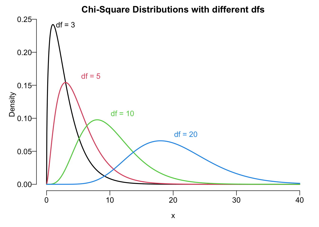
As Student’s $t$ distribution, the chi-square $χ^{2}$ distribution has one parameter, degrees of freedom $d f$ . To denote a specific chi-square distribution, we write $χ_{d f}^{2}$ like $χ_{2}^{2}$ for a chi-square distribution or variable with degrees of freedom two. Figure 18.1 shows $χ^{2}$ distributions with varying degrees of freedom. It is in general a right-skewed distribution, but it gets more and more symmetric as $d f$ gets larger. Also, the $χ^{2}$ distribution is defined over positive numbers, one hint why we use it for inferring variances because variance is non-negative, but normal or $t$ distribution is defined on the whole real line.

Figure 18.1: Illustration of $χ^{2}$ distributions with varying degrees of freedom

viewof params = Inputs.form([
      Inputs.range([1, 100], {value: 4, step: 1, label: tex`\nu`}),
      Inputs.range([0.01, 50], {value: 2, step: 0.01, label: "quantile:"})
    ])

params = Array(2) [4, 2]

dist_quantile = tex`\text{If } X \sim \chi^2_{${params[0]}} \text{ then } `

\text{If } X \sim \chi^2_{4} \text{ then }

moments = tex`
\begin{aligned}
&E( X) =\nu = ${params[0].toPrecision(3)} \\[1em]
&Var( X) =2\nu= ${(2*params[0]).toPrecision(3)} \\[1em]
&P( X\leq ${params[1]}) =${chisquarecdf.toPrecision(4)}
\end{aligned}
`

\begin{aligned} &E( X) =\nu = 4.00 \\[1em] &Var( X) =2\nu= 8.00 \\[1em] &P( X\leq 2) =0.2642 \end{aligned}

plt_pdf = Plot.plot({
    color: {
      legend: true
    },
    x: {
      label: "x",
      axis: true
    },
    y: {
      label: "f(x)",
      //axis: false,
      domain: [0,jstat.chisquare.pdf(Math.max(0,params[0]-2), params[0])]
    },
    marks: [
      Plot.ruleY([0]),
      Plot.ruleX([0]),
      Plot.line(chisquarepdf, {x: "x", y: "pdf", stroke : "steelblue", strokeWidth: 2}),
      Plot.areaY(chisquarepdf, {filter: d => d.x <= params[1], x: "x", y: "pdf", fill: "steelblue", opacity: 0.2})
    ]
  })

Figure 18.2: Source: https://observablehq.com/@mattiasvillani/chi2-distribution

chisquarepdf = {
  const x = d3.range(0.01, params[0]+5*Math.sqrt(2*params[0]), 0.01);
  const pdf = x.map(x => ({x: x, pdf: jstat.chisquare.pdf(x, params[0])}));
  return pdf
}

chisquarepdf = Array(1814) [Object, Object, Object, Object, Object, Object, Object, Object, Object, Object, Object, Object, Object, Object, Object, Object, Object, Object, Object, Object, …]

chisquarecdf = jstat.chisquare.cdf(params[1], params[0]);

chisquarecdf = 0.2642411176571154

jstat = require('jstat')

jstat = ƒ()

Upper Tail and Lower Tail of Chi-Square

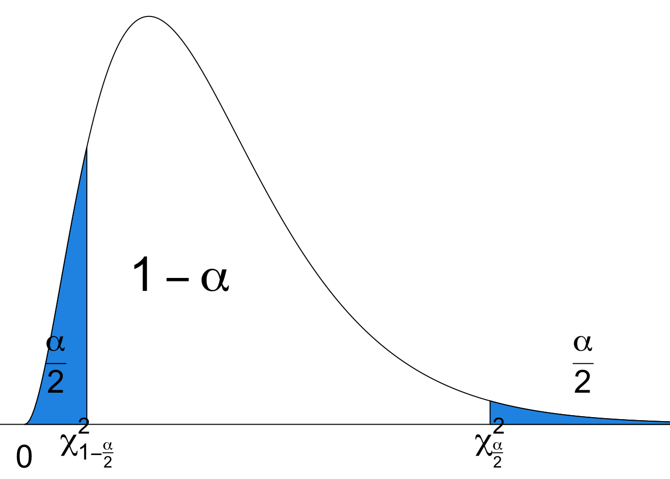
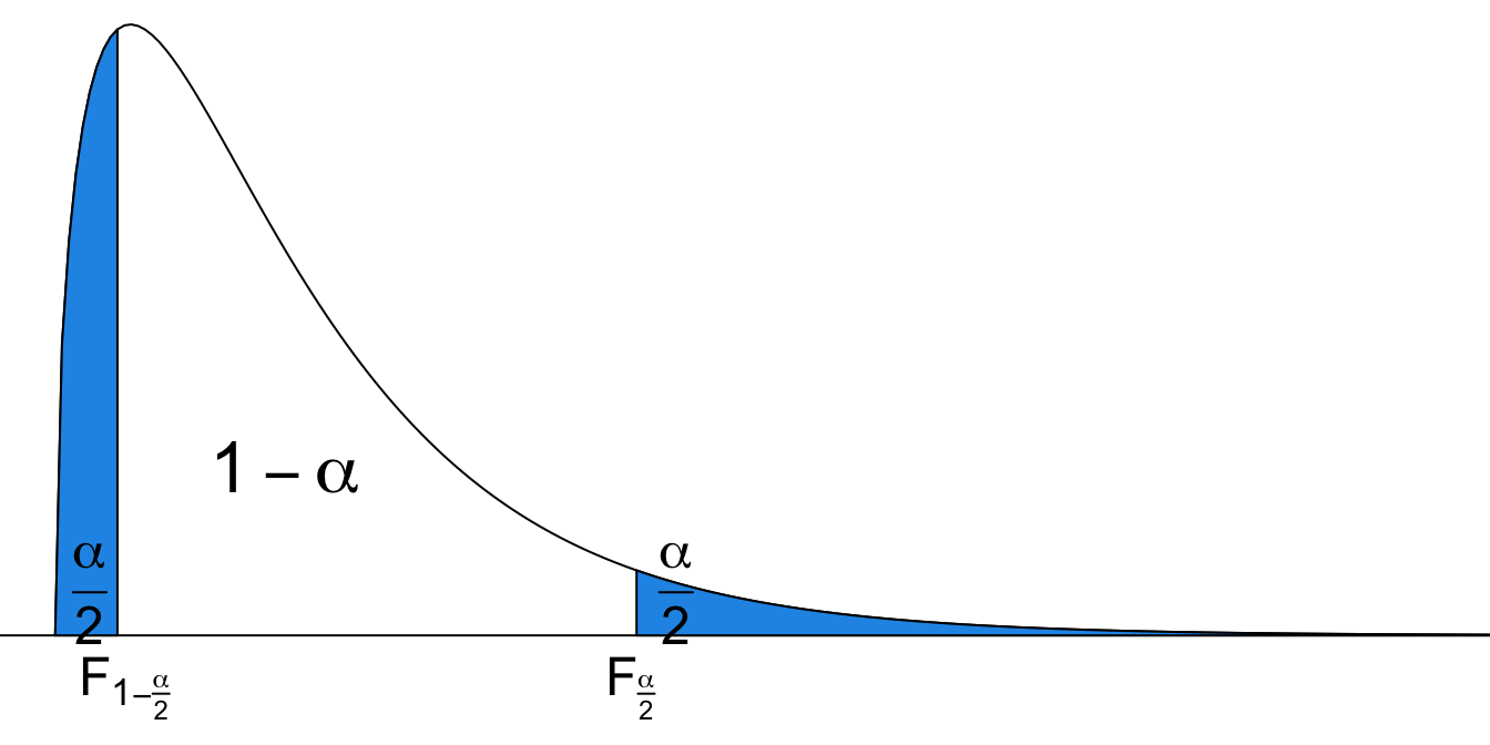
Like standard normal and $t$ distribution, to do the inference for variances, we get to find or define critical values of a chi-square distribution. With some probability $α$ , we define

$χ_{\frac{α}{2}, d f}^{2}$ is a $χ^{2}$ value of a $χ^{2}$ distribution with degrees of freedom $d f$ such that it has area to the right of $α / 2$ .
$χ_{1 - \frac{α}{2}, d f}^{2}$ is a $χ^{2}$ value of a $χ^{2}$ distribution with degrees of freedom $d f$ such that it has area to the left of $α / 2$ . In other words, it has area to the right of $1 - α / 2$ , and that’s why it has a subscript $1 - \frac{α}{2}$ .

Figure 18.3 illustrates the $χ^{2}$ critical values. Notice that in $N (0, 1)$ , $z_{1 - \frac{α}{2}} = - z_{\frac{α}{2}}$ . Because of the symmetry of the distribution, the $z$ -value having area $α / 2$ on the right is the $z$ -value having area $α / 2$ on the left with a negative sign. However, the chi-square distribution is not symmetric, so $χ_{1 - \frac{α}{2}, d f}^{2} \neq - χ_{\frac{α}{2}, d f}^{2}$ .

Figure 18.3: Illustration of $α / 2$ significance levels for $χ_{d f}^{2}$ distribution

Sampling Distribution

When a random sample of size $n$ is from $N (μ, σ^{2})$ , the following sample statistic has the $χ^{2}$ sampling distribution with degrees of freedom $n - 1$ : $\frac{(n - 1) S^{2}}{σ^{2}} \sim χ_{n - 1}^{2} .$

I would like to stress again that the inference method for $σ^{2}$ introduced here can work poorly if the normality assumption is violated, even for large samples.

The sample statistic involves $S^{2}$ and $σ^{2}$ , so we have manipulate its sampling distribution to obtain the confidence interval for $σ^{2}$ , and use it as a test statistic in the hypothesis testing for $σ^{2}$ .

$(1 - α) 100 %$ Confidence Interval for $σ^{2}$

The $(1 - α) 100 %$ confidence interval for $σ^{2}$ is $(\frac{(n - 1) S^{2}}{χ_{\frac{α}{2}, n - 1}^{2}}, \frac{(n - 1) S^{2}}{χ_{1 - \frac{α}{2}, n - 1}^{2}})$

How do we get this interval? We start with the sampling distribution of $\frac{(n - 1) S^{2}}{σ^{2}}$ .

$P (χ_{1 - \frac{α}{2}, n - 1}^{2} < \frac{(n - 1) S^{2}}{σ^{2}} < χ_{\frac{α}{2}, n - 1}^{2}) = 1 - α$ (Goal: isolate $σ^{2}$ )
$P (\frac{χ_{1 - \frac{α}{2}, n - 1}^{2}}{(n - 1) S^{2}} < \frac{1}{σ^{2}} < \frac{χ_{\frac{α}{2}, n - 1}^{2}}{(n - 1) S^{2}}) = 1 - α$ (divided by $(n - 1) S^{2}$ )
$P (\frac{(n - 1) S^{2}}{χ_{1 - \frac{α}{2}, n - 1}^{2}} > σ^{2} > \frac{(n - 1) S^{2}}{χ_{\frac{α}{2}, n - 1}^{2}}) = 1 - α$ (take reciprocal)
$P (\frac{(n - 1) S^{2}}{χ_{\frac{α}{2}, n - 1}^{2}} < σ^{2} < \frac{(n - 1) S^{2}}{χ_{1 - \frac{α}{2}, n - 1}^{2}}) = 1 - α$ (smaller value on the left)

Be careful that the interval for $σ^{2}$ cannot be expressed as $(S^{2} - m, S^{2} + m)$ for some margin of error $m$ anymore!

Example: Supermodel Heights

Listed below are heights (cm) for the simple random sample of 16 female supermodels.

R
Python

heights <- c(178, 177, 176, 174, 175, 178, 175, 178, 
             178, 177, 180, 176, 180, 178, 180, 176)

import numpy as np
heights = np.array([178, 177, 176, 174, 175, 178, 175, 178, 
             178, 177, 180, 176, 180, 178, 180, 176])

The supermodels’ heights are normally distributed. Please construct a $95 %$ confidence interval for population standard deviation $σ$ .

We just need to get what we need for constructing the interval from the sample data, sample size $n$ , sample variance $s^{2}$ , $α$ , critical values $χ_{α / 2, n - 1}^{2}$ and $χ_{1 - α / 2, n - 1}^{2}$ .

$n = 16$ , $s^{2} = 3.4$ , $α = 0.05$ .
$χ_{α / 2, n - 1}^{2} = χ_{0.025, 15}^{2} = 27.49$
$χ_{1 - α / 2, n - 1}^{2} = χ_{0.975, 15}^{2} = 6.26$

Note that we want the interval for $σ$ , not $σ^{2}$ , we take a square root of the lower and upper bound of the interval for $σ^{2}$ . The $95 %$ CI for $σ$ is $(\sqrt{\frac{(n - 1) s^{2}}{χ_{\frac{α}{2}, n - 1}^{2}}}, \sqrt{\frac{(n - 1) s^{2}}{χ_{1 - \frac{α}{2}, n - 1}^{2}}}) = (\sqrt{\frac{(16 - 1) (3.4)}{27.49}}, \sqrt{\frac{(16 - 1) (3.4)}{6.26}}) = (1.36, 2.85)$

We are 95% confident that the height of supermodels has standard deviation between 1.36 and 2.85.

R
Python

We use qchisq() to get the $χ^{2}$ critical values. The probability $p$ and the degrees of freedom df need to be specified. You should be able to understand the rest part of the code. Enjoy it.

## set values
n <- 16
s2 <- var(heights)
alpha <- 0.05

## two chi-square critical values
chi2_right <- qchisq(p = alpha/2, df = n - 1, lower.tail = FALSE)
chi2_left <- qchisq(p = alpha/2, df = n - 1, lower.tail = TRUE)

## two bounds of CI for sigma2
ci_sig2_lower <- (n - 1) * s2 / chi2_right
ci_sig2_upper <- (n - 1) * s2 / chi2_left

## two bounds of CI for sigma
(ci_sig_lower <- sqrt(ci_sig2_lower))

[1] 1.362104

(ci_sig_upper <- sqrt(ci_sig2_upper))

[1] 2.853802

import numpy as np
from scipy.stats import chi2

We use chi2 family in scipy.stats to get the $χ^{2}$ critical values. The probability $p$ and the degrees of freedom df need to be specified. You should be able to understand the rest part of the code. Enjoy it.

# Set values
n = 16
s2 = np.var(heights, ddof=1)  # sample variance
alpha = 0.05

# Chi-square critical values
chi2_right = chi2.isf(alpha/2, df=n-1)
chi2_left = chi2.ppf(alpha/2, df=n-1)

# Confidence interval for variance (sigma^2)
ci_sig2_lower = (n - 1) * s2 / chi2_right
ci_sig2_upper = (n - 1) * s2 / chi2_left

# Confidence interval for standard deviation (sigma)
ci_sig_lower = np.sqrt(ci_sig2_lower)
ci_sig_lower

1.3621044553698662

ci_sig_upper = np.sqrt(ci_sig2_upper)
ci_sig_upper

2.8538016067984957

Testing

Back to the example. Use $α = 0.05$ to test the claim that “supermodels have heights with a standard deviation that is less than the standard deviation, $σ = 7.5$ cm, for the population of women”.

Step 1

We are comparing the $σ$ of heights of supermodels with the $σ$ of heights of women in general which is 7.5. So the hypothesize value $σ_{0}$ is 7.5. We wonder if supermodel height standard deviation is smaller than 7.5. Therefore, we have test $H_{0} : σ = σ_{0}$ vs. $H_{1} : σ < σ_{0}$ , where $σ_{0} = 7.5$ cm.

Step 2

$α = 0.05$

Step 3

The test statistic comes from the variable $χ_{t e s t}^{2} = \frac{(n - 1) S^{2}}{σ^{2}}$ that follows $χ_{n - 1}^{2}$ distribution. Under $H_{0}$ , we have $χ_{t e s t}^{2} = \frac{(n - 1) s^{2}}{σ_{0}^{2}} = \frac{(16 - 1) (3.4)}{{7.5}^{2}} = 0.91$ , drawn from $χ_{n - 1}^{2}$ .

Step 4-c

This is a left-tailed test.
The critical value is $χ_{1 - α, d f}^{2} = χ_{0.95, 15}^{2} = 7.26$

Step 5-c

Reject $H_{0}$ in favor of $H_{1}$ if $χ_{t e s t}^{2} < χ_{1 - α, d f}^{2}$ .
Since $0.91 < 7.26$ , we reject $H_{0}$ .

Step 6

There is sufficient evidence to support the claim that supermodels have heights with a standard deviation that is less than the standard deviation for the population of all women.

We conclude that the heights of supermodels vary less than heights of women in the general women population.

Back to Pooled t-Test

In a two sample pooled t-test, we assume

$n_{1} \geq 30$ and $n_{2} \geq 30$ or that both samples are drawn from normal populations.
$σ_{1} = σ_{2}$

We can use a QQ-plot (and normality tests, Anderson, Shapiro, etc.) to check the assumption of a normal distribution. We now learn how to check the assumption $σ_{1} = σ_{2}$ .

18.2 Inference for Comparing Two Population Variances

F Distribution

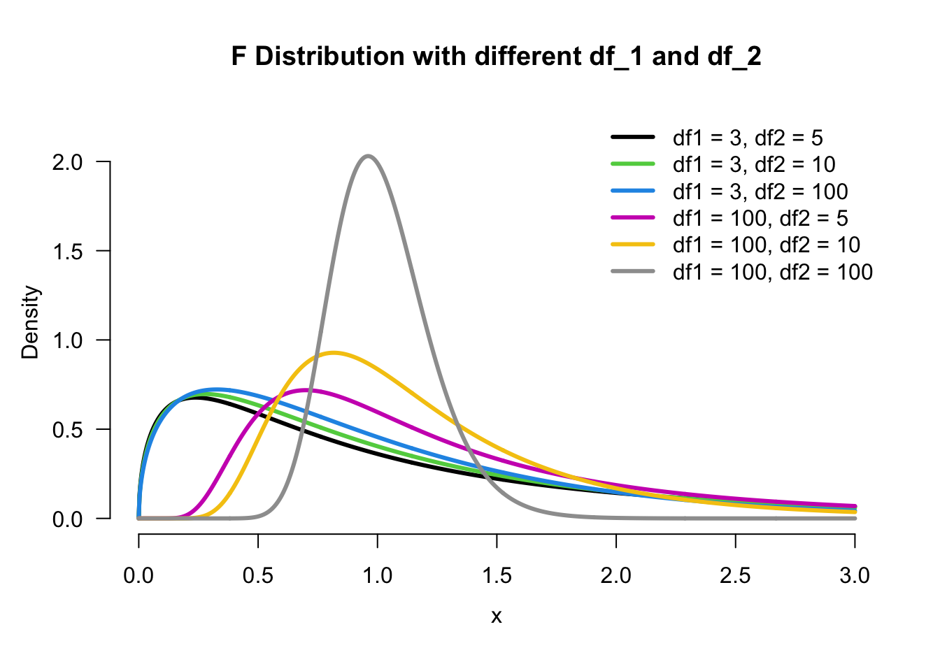
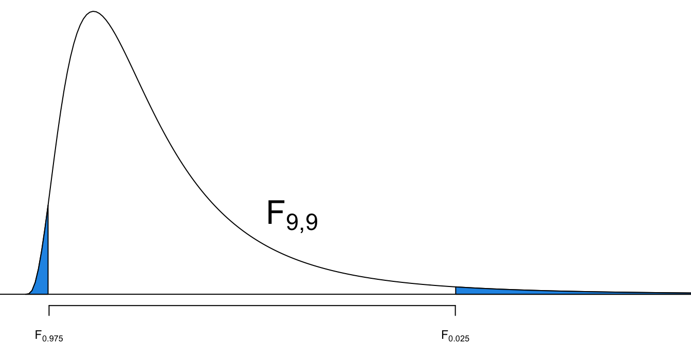
For comparing two population variances, we need another distribution called $F$ distribution. The $F$ distribution has two parameters $d f_{1}$ and $d f_{2}$ , a hint why it is used for comparing two variances. We write a specific $F$ distribution $F_{d f_{1}, d f_{2}}$ . Second, the $F$ distribution is also right-skewed. Like $χ^{2}$ distribution, the $F$ distribution is defined over positive numbers. Figure 18.4 illustrates $F$ distribution with different parameters. You can see that when $d f_{1}$ and $d f_{2}$ are both large, the $F$ distribution looks bell-shaped.

viewof params_f = Inputs.form([
      Inputs.range([1, 100], {value: 4, step: 1, label: tex`\nu_1`}),
      Inputs.range([1, 100], {value: 4, step: 1, label: tex`\nu_2`}),
      Inputs.range([0.01, 10], {value: 2, step: 0.01, label: "quantile:"})
    ])

params_f = Array(3) [4, 4, 2]

dist_quantile_f = tex`\text{If } X \sim F(${nu1},${nu2}) \text{ then } `

\text{If } X \sim F(4,4) \text{ then }

moments_f = {
  if (nu2>4){
    return tex`
      \begin{aligned}
        &E( X) =\frac{\nu_2}{\nu_2-2} = ${(nu2/(nu2-2)).toPrecision(3)} \\[1em]
        &Var( X) = 2\Big(\frac{\nu_2}{\nu_2-2}\Big)^2\frac{\nu_1+\nu_2-2}{\nu_1(\nu_2-4)} = 
        ${(2*(nu2/(nu2-2))**2 * ((nu1+nu2-2)/(nu1*(nu2-4)))).toPrecision(3)} \\[1em]
        &P( X\leq ${quantile}) =${fcdf.toPrecision(4)}
      \end{aligned}
    `
  }
  else{
    if (nu2>2 && nu2<=4){
      return tex`
      \begin{aligned}
        &E( X) =\frac{\nu_2}{\nu_2-2} = ${(nu2/(nu2-2)).toPrecision(3)} ( \nu_2>2 \text{ is needed} )\\[1em]
        &Var( X) = \text{ does not exist} ( \nu_2>4 \text{ is needed} ) \\[1em]
        &P( X\leq ${quantile}) =${fcdf.toPrecision(4)}
      \end{aligned}
    `
    }
    else{
    return tex`
      \begin{aligned}
        &E( X) =\text{ does not exist} ( \nu_2>2 \text{ is needed} )\\[1em]
        &Var( X) = \text{ does not exist} ( \nu_2>4 \text{ is needed} ) \\[1em]
        &P( X\leq ${quantile}) =${fcdf.toPrecision(4)}
      \end{aligned}
    `
    }
  }
  
}

\begin{aligned} &E( X) =\frac{\nu_2}{\nu_2-2} = 2.00 ( \nu_2>2 \text{ is needed} )\\[1em] &Var( X) = \text{ does not exist} ( \nu_2>4 \text{ is needed} ) \\[1em] &P( X\leq 2) =0.7407 \end{aligned}

plt_pdf_f = Plot.plot({
    color: {
      legend: true
    },
    x: {
      label: "x",
      axis: true
    },
    y: {
      label: "f(x)",
      //axis: false,
      //domain: [0,jstat.chisquare.pdf(mode, nu1, nu2)]
    },
    marks: [
      Plot.ruleY([0]),
      Plot.ruleX([0]),
      Plot.line(fpdf, {x: "x", y: "pdf", stroke : "purple", strokeWidth: 2}),
      Plot.areaY(fpdf, {filter: d => d.x <= quantile, x: "x", y: "pdf", fill: "purple", opacity: 0.2})
    ]
  })

Figure 18.5: Source: https://observablehq.com/@mattiasvillani/f-distribution

nu1 = params_f[0]
nu2 = params_f[1]
quantile = params_f[2]

nu1 = 4

nu2 = 4

quantile = 2

fpdf = {
  const x = d3.range(0.01, jstat.centralF.inv( 0.99, nu1, nu2 ), 0.01);
  const pdf = x.map(x => ({x: x, pdf: jstat.centralF.pdf(x, nu1, nu2 )}));
  return pdf
}

fpdf = Array(1597) [Object, Object, Object, Object, Object, Object, Object, Object, Object, Object, Object, Object, Object, Object, Object, Object, Object, Object, Object, Object, …]

fcdf = jstat.centralF.cdf(quantile, nu1, nu2);

fcdf = 0.7407407407407405

Upper and Lower Tail of F Distribution

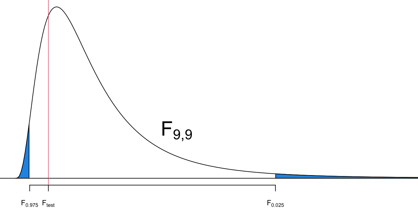
We denote $F_{α, d f_{1}, d f_{2}}$ as the $F$ quantile such that $P (F_{d f_{1}, d f_{2}} > F_{α, d f_{1}, d f_{2}}) = α$ . With it, we can find the critical values $F_{\frac{α}{2}, d f_{1}, d f_{2}}$ and $F_{1 - \frac{α}{2}, d f_{1}, d f_{2}}$ used in constructing the confidence interval for the ratio $σ_{1}^{2} / σ_{2}^{2}$ discussed next.

Figure 18.6: Illustration of $α / 2$ significance levels for $F_{d f_{1}, d f_{2}}$ distribution

Sampling Distribution

When random samples of sizes $n_{1}$ and $n_{2}$ have been independently drawn from two normally distributed populations, $N (μ_{1}, σ_{1}^{2})$ and $N (μ_{2}, σ_{2}^{2})$ respectively, the ratio $\frac{S_{1}^{2} / S_{2}^{2}}{σ_{1}^{2} / σ_{2}^{2}}$ has the $F$ sampling distribution $\frac{S_{1}^{2} / S_{2}^{2}}{σ_{1}^{2} / σ_{2}^{2}} \sim F_{n_{1} - 1, n_{2} - 1} .$

Important

The order of degrees of freedom matters! $F_{n_{1} - 1, n_{2} - 1} \neq F_{n_{2} - 1, n_{1} - 1}$ . Please don’t mess around.

$(1 - α) 100 %$ Confidence Interval for $σ_{1}^{2} / σ_{2}^{2}$

From the sampling distribution of the ratio, the $(1 - α) 100 %$ confidence interval for $σ_{1}^{2} / σ_{2}^{2}$ is $(\frac{s_{1}^{2} / s_{2}^{2}}{F_{α / 2, n_{1} - 1, n_{2} - 1}}, \frac{s_{1}^{2} / s_{2}^{2}}{F_{1 - α / 2, n_{1} - 1, n_{2} - 1}})$

How do we get the interval? Not surprising. We start with the sampling distribution of $\frac{S_{1}^{2} / S_{2}^{2}}{σ_{1}^{2} / σ_{2}^{2}}$ .

$P (F_{1 - α / 2, n_{1} - 1, n_{2} - 1} < \frac{S_{1}^{2} / S_{2}^{2}}{σ_{1}^{2} / σ_{2}^{2}} < F_{α / 2, n_{1} - 1, n_{2} - 1}) = 1 - α$ (Goal: isolate $σ_{1}^{2} / σ_{2}^{2}$ )
$P (\frac{1}{F_{α / 2, n_{1} - 1, n_{2} - 1}} < \frac{σ_{1}^{2} / σ_{2}^{2}}{S_{1}^{2} / S_{2}^{2}} < \frac{1}{F_{1 - α / 2, n_{1} - 1, n_{2} - 1}}) = 1 - α$ (take reciprocal)
$P (\frac{S_{1}^{2} / S_{2}^{2}}{F_{α / 2, n_{1} - 1, n_{2} - 1}} < \frac{σ_{1}^{2}}{σ_{2}^{2}} < \frac{S_{1}^{2} / S_{2}^{2}}{F_{1 - α / 2, n_{1} - 1, n_{2} - 1}}) = 1 - α$ (times $S_{1}^{2} / S_{2}^{2}$ )

Note

The confidence interval for $σ_{1}^{2} / σ_{2}^{2}$ cannot be expressed as $(\frac{s_{1}^{2}}{s_{2}^{2}} - m, \frac{s_{1}^{2}}{s_{2}^{2}} + m)$ anymore!

F test for comparing $σ_{1}^{2}$ and $σ_{2}^{2}$

Step 1

For comparing $σ_{1}^{2}$ and $σ_{2}^{2}$ , the test can be either right-tailed or two-tailed. Left-tailed testing is not necessary because we can always define the population whose variance is hypothetically larger than the variance of another population as the first population.

Right-tailed: $\begin{aligned} H_{0} : σ_{1} \leq σ_{2} \\ H_{1} : σ_{1} > σ_{2} \end{aligned}$
Two-tailed: $\begin{aligned} H_{0} : σ_{1} = σ_{2} \\ H_{1} : σ_{1} \neq σ_{2} \end{aligned}$

Step 2

$α = 0.05$

Step 3

Under $H_{0}$ , $σ_{1} = σ_{2}$ , and the test statistic is $F_{t e s t} = \frac{s_{1}^{2} / s_{2}^{2}}{σ_{1}^{2} / σ_{2}^{2}} = \frac{s_{1}^{2}}{s_{2}^{2}} \sim F_{n_{1} - 1, n_{2} - 1}$ The denominator is gone because the ratio is one.

Step 4-c

Right-tailed: $F_{α, n_{1} - 1, n_{2} - 1}$ .
Two-tailed: $F_{α / 2, n_{1} - 1, n_{2} - 1}$ or $F_{1 - α / 2, n_{1} - 1, n_{2} - 1}$

Step 5-c

Right-tailed: reject $H_{0}$ if $F_{t e s t} \geq F_{α, n_{1} - 1, n_{2} - 1}$ .
Two-tailed: reject $H_{0}$ if $F_{t e s t} \geq F_{α / 2, n_{1} - 1, n_{2} - 1}$ or $F_{t e s t} \leq F_{1 - α / 2, n_{1} - 1, n_{2} - 1}$

Example: Weight Loss

This is our previous example.

A study was conducted to see the effectiveness of a weight loss program. Two groups (Control and Experimental) of 10 subjects were selected. The two populations are normally distributed and have the same standard deviation.

The data on weight loss was collected at the end of six months.

Control: $n_{1} = 10$ , ${\overset{―}{x}}_{1} = 2.1 l b$ , $s_{1} = 0.5 l b$
Experimental: $n_{2} = 10$ , ${\overset{―}{x}}_{2} = 4.2 l b$ , $s_{2} = 0.7 l b$

Check if $σ_{1} = σ_{2}$

$n_{1} = 10$ , $s_{1} = 0.5 l b$
$n_{2} = 10$ , $s_{2} = 0.7 l b$

Step 1

$\begin{aligned} H_{0} : σ_{1} = σ_{2} \\ H_{1} : σ_{1} \neq σ_{2} \end{aligned}$

Step 2

$α = 0.05$

Step 3

The test statistic is $F_{t e s t} = \frac{s_{1}^{2}}{s_{2}^{2}} = \frac{{0.5}^{2}}{{0.7}^{2}} = 0.51$ .

Step 4-c

This is a two-tailed test.
The critical value is $F_{0.05 / 2, 10 - 1, 10 - 1} = 4.03$ or $F_{1 - 0.05 / 2, 10 - 1, 10 - 1} = 0.25$ .

Step 5-c

Is $F_{t e s t} > 4.03$ or $F_{t e s t} < 0.25$ ?
- No.

Step 6

The evidence is not sufficient to reject the claim that $σ_{1} = σ_{2}$ .

95% CI for $σ_{1}^{2} / σ_{2}^{2}$

$F_{α / 2, d f_{1}, d f_{2}} = F_{0.05 / 2, 10 - 1, 10 - 1} = 4.03$
$F_{1 - α / 2, d f_{1}, d f_{2}} = F_{1 - 0.05 / 2, 10 - 1, 10 - 1} = 0.25$
$\frac{s_{1}^{2}}{s_{2}^{2}} = \frac{{0.5}^{2}}{{0.7}^{2}} = 0.51$
The 95% CI for $σ_{1}^{2} / σ_{2}^{2}$ is $\begin{aligned} (\frac{s_{1}^{2} / s_{2}^{2}}{F_{α / 2, d f_{1}, d f_{2}}}, \frac{s_{1}^{2} / s_{2}^{2}}{F_{1 - α / 2, d f_{1}, d f_{2}}}) \\ = (\frac{0.51}{4.03}, \frac{0.51}{0.25}) = (0.127, 2.05) \end{aligned}$

We are 95% confident that the ratio $σ_{1}^{2} / σ_{2}^{2}$ is between 0.127 and 2.04. Because one is included in this interval, meaning that $σ_{1}^{2} = σ_{2}^{2}$ , it leads to the same conclusion as the F test.

R
python

We use qf() to find the $F$ critical values.

## set values
n1 <- 10; n2 <- 10
s1 <- 0.5; s2 <- 0.7
alpha <- 0.05

## 95% CI for sigma_1^2 / sigma_2^2
f_small <- qf(p = alpha / 2, df1 = n1 - 1, df2 = n2 - 1,lower.tail = TRUE)
f_big <- qf(p = alpha / 2, df1 = n1 - 1, df2 = n2 - 1, lower.tail = FALSE)

## lower bound
(s1 ^ 2 / s2 ^ 2) / f_big

[1] 0.1267275

## upper bound
(s1 ^ 2 / s2 ^ 2) / f_small

[1] 2.054079

## Testing sigma_1 = sigma_2
(test_stats <- s1 ^ 2 / s2 ^ 2)

[1] 0.5102041

We use f.ppf() and f.isf() in scipy.stats to find the $F$ critical values.

from scipy.stats import f

# Set values
n1 = 10; n2 = 10
s1 = 0.5; s2 = 0.7
alpha = 0.05

# F-distribution critical values
f_small = f.ppf(alpha/2, dfn=n1-1, dfd=n2-1)
f_big = f.isf(alpha/2, dfn=n1-1, dfd=n2-1)

# Confidence interval for the ratio of variances (sigma_1^2 / sigma_2^2)
# lower bound
(s1**2/s2**2)/f_big

0.126727476884926

# upper bound
(s1**2/s2**2)/f_small

2.054078652185193

# F-test statistic
test_stats = (s1**2)/(s2**2)
test_stats

0.5102040816326532

Note

If we have the entire two samples data, we can use the R built-in function var.test(x, y, alternative = "two.sided") to perform a $F$ test to compare the variances of two samples from normal populations. The arguments x and y are numeric vectors of data values. Argument alternative must be one of "two.sided" (default), "greater" or "less".

18.3 Comparing More Than Two Population Variances*

So far we use $χ^{2}$ distribution to do inference for one population variance, and $F$ distribution to compare two variances. What if we want to compare more than two population variances? For example, what do we do if we have this kind of test:

$\begin{aligned} H_{0} : σ_{1} = σ_{2} = \dots = σ_{t} \\ H_{1} : Population variances are not all equal \end{aligned}$

where we have $t > 2$ different groups. In this scenario, we can use the so-called Brown-Forsythe-Levene (BFL) test. The BFL test assumes that we have $t > 2$ independent samples. Then BFL replaces $y_{i j}$ , the $j$ -th observation in group $i$ , with $z_{i j}$ . $z_{i j} = | y_{i j} - {\tilde{y}}_{i} |$ , where ${\tilde{y}}_{i}$ is the sample median or mean of group $i$ .

Note

Brown-Forsythe-Levene test actually represents two tests: Brown-Forsythe test and Levene’s test, where Brown-Forsythe test uses the sample medians in $z_{i j}$ and Levene’s test uses the sample means. This is the only difference between the two tests, and therefore some will refer them as one Brown-Forsythe-Levene test, or some even refer one to the other. For example, the R function car::leveneTest() used in the example actually perform the Brown-Forsythe test by default with its argument center=median.

Using means has larger statistical power for symmetric, moderate-tailed, distributions. But when data are non-normal, either skewed or heavy tailed, using medians is recommended because of good robustness against many types of non-normal data and while retaining good statistical power.

The test statistic is $L_{t e s t} = \frac{\sum_{i = 1}^{t} n_{i} ({\overset{―}{z}}_{i \cdot} - {\overset{―}{z}}_{\cdot \cdot})^{2} / (t - 1)}{\sum_{i = 1}^{t} \sum_{j = 1}^{n_{i}} (z_{i j} - {\overset{―}{z}}_{i \cdot})^{2} / (N - t)}$ , where ${\overset{―}{z}}_{i \cdot} = \sum_{j = 1}^{n_{i}} z_{i j} / n_{i}$ is the mean of the $z_{i j}$ s from the group $i$ , ${\overset{―}{z}}_{\cdot \cdot} = \sum_{i = 1}^{t} \sum_{j = 1}^{n_{i}} z_{i j} / N$ is the mean of all $z_{i j}$ s, and $N = \sum_{i = 1}^{t} n_{i}$ .

The decision rule is that we reject $H_{0}$ if $L_{t e s t} > F_{α, t - 1, N - t}$ .

There are other tests for testing the homogeneity of variances, but the BFL test performs better when data are from a non-normal distribution. It corrects for the skewness of distribution by using deviations from group medians. The BFL test is more robust. It is less likely to incorrectly declare that the assumption of equal variances has been violated.

Example: Automobile Additives (Example 7.8 in SMD)

Three different additives that are marketed for increasing the miles per gallon (mpg) for automobiles. The percentage increase in mpg was recorded for a 250-mile test drive for each additive for 10 randomly assigned cars. Is there a difference between the three additives with respect to their variability?

R
Python

The data are saved in R data frame data_additive.

data_additive

   mpg_increase additive
1           4.2        1
2           2.9        1
3           0.2        1
4          25.7        1
5           6.3        1
6           7.2        1
7           2.3        1
8           9.9        1
9           5.3        1
10          6.5        1
11          0.2        2
12         11.3        2
13          0.3        2
14         17.1        2
15         51.0        2
16         10.1        2
17          0.3        2
18          0.6        2
19          7.9        2
20          7.2        2
21          7.2        3
22          6.4        3
23          9.9        3
24          3.5        3
25         10.6        3
26         10.8        3
27         10.6        3
28          8.4        3
29          6.0        3
30         11.9        3

The data are saved in Python pd.DataFrame data_additive.

    mpg_increase additive
0            4.2        1
1            2.9        1
2            0.2        1
3           25.7        1
4            6.3        1
5            7.2        1
6            2.3        1
7            9.9        1
8            5.3        1
9            6.5        1
10           0.2        2
11          11.3        2
12           0.3        2
13          17.1        2
14          51.0        2
15          10.1        2
16           0.3        2
17           0.6        2
18           7.9        2
19           7.2        2
20           7.2        3
21           6.4        3
22           9.9        3
23           3.5        3
24          10.6        3
25          10.8        3
26          10.6        3
27           8.4        3
28           6.0        3
29          11.9        3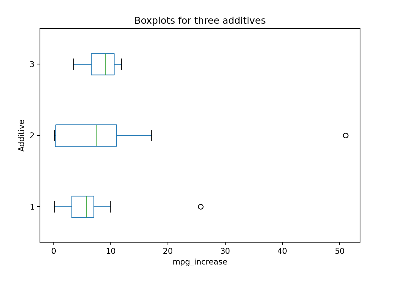

The boxplot suggests that Additive 2 has larger variation than the other two in terms of the percentage increase in mpg. We will use the BFL test to decide whether or not their variation difference is just a random sampling consequences or it is statistically significant.

The procedure of BLT test is shown step by step as follows.

Step 1: $\begin{aligned} H_{0} : σ_{1} = σ_{2} = σ_{3} \\ H_{1} : Population variances are not all equal \end{aligned}$
Step 2: $α = 0.05$
Step 3: Test statistic $L_{t e s t} = \frac{\sum_{i = 1}^{t} n_{i} ({\overset{―}{z}}_{i \cdot} - {\overset{―}{z}}_{\cdot \cdot})^{2} / (t - 1)}{\sum_{i = 1}^{t} \sum_{j = 1}^{n_{i}} (z_{i j} - {\overset{―}{z}}_{i \cdot})^{2} / (N - t)} = \frac{235.8 / (3 - 1)}{1742.6 / (30 - 3)} = 1.872$ .
Step4-c: Critical value is $F_{α, t - 1, N - t} = F_{0.05, 3 - 1, 30 - 3} = 3.35$ .
Step5-c: Since $L_{t e s t} = 1.872 < F_{α, t - 1, N - t} = 3.35$ , we do not reject $H_{0}$ .
Step6: There is insufficient evidence to support the claim that there is a difference in the population variances of the percentage increase in mpg for the three additives.

R
Python

Once you understand the idea and the process of doing the test, in practice, we use R function leveneTest() in the car (Companion to Applied Regression) package to help us perform the test.

library(car) # Load the package car
leveneTest(y = data_additive$mpg_increase, 
           group = data_additive$additive)

Levene's Test for Homogeneity of Variance (center = median)
      Df F value Pr(>F)
group  2  1.8268 0.1803
      27

In the function, we put the response variable data in y, and the factor defining groups in group. By default, it will use sample medians to perform the test. The p-value is greater than 0.05 and it leads to the same conclusion that there is insufficient evidence to say there is a difference in the population variances of the percentage increase in mpg for the three additives.

Once you understand the idea and the process of doing the test, in practice, we use Python function levene() in scipy.stats to help us perform the test.

from scipy.stats import levene
# Levene's test
levene(
    data_additive[data_additive['additive'] == 1]['mpg_increase'],
    data_additive[data_additive['additive'] == 2]['mpg_increase'],
    data_additive[data_additive['additive'] == 3]['mpg_increase'])

LeveneResult(statistic=1.82684271595955, pvalue=0.18025794484918528)

In the function, each sample data can only be one-dimensional. By default, it will use sample medians to perform the test. The p-value is greater than 0.05 and it leads to the same conclusion that there is insufficient evidence to say there is a difference in the population variances of the percentage increase in mpg for the three additives.

18.4 Exercises

The data about male and female pulse rates are summarized below.
1. Construct a 95% CI for $σ_{m a l e}$ of pulse rates for males.
2. Construct a 95% CI for $σ_{m a l e} / σ_{f e m a l e}$ .
3. Does it appear that the population standard deviations for males and females are different? Why or why not?

	Male	Female
$\overset{―}{x}$	71	75
$s$	9	12
$n$	14	12