9 Random Variables
In this chapter, we talk about random variables, an important idea that connects our sample data points to probability.
9.1 Random Variables
In Chapter 2, we learn that a variable in a data set is a characteristic or attribute that varies from one object to another. A variable can be either categorical or numerical. For example, gender is categorical and height is numerical. In addition, numerical variables can be either discrete or continuous. A discrete variable takes on values of a finite or countable number, while a continuous variable takes on values anywhere over a particular range without gaps or jumps. So the number of conferences Dr. Yu attended last year is discrete, and college GPA is continuous.
We know variables in a data set vary from one to another. If a variable takes numerical values, and its value is determined by some chance or randomness of a procedure or experiment, then we say the variable is a random variable, usually denoted as \(X\) or other capital English letters, \(Y\), \(Z\) for example.
Usually a capital letter represents a random variable and a small letter represents a realized value of that random variable. For example, \(X\) is weight which is a random variable, and \(x\) is a realized value of \(X\) that can be any possible value of \(X\), for example, \(X = 170\) means the realized value \(x\) is 170.
Other random variable examples are
\(X\) = # of heads after flipping a coin twice.
\(X\) = # of accidents in W. Wisconsin Ave. per day
Note that \(X\) must follow some randomness pattern, and its realized value cannot be known in advance unless we collect the data or realize it.
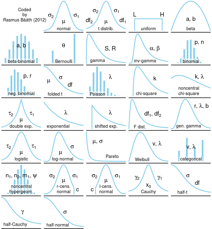
To accounting for its randomness, a random variable has a probability distribution associated with it. The probability distribution governs the behavior of the random variable, indicating the range of the possible values, and what values are more probable to be realized than others. Probability distribution is key to uncertainty quantification in statistical inference and machine learning prediction. Figure 9.1 below shows the many different types of probability distributions, and we’ll discuss a few basic but important probability distributions in Chapter 10 and Chapter 11.
When a random variable is defined, \(X = x\) or \(a < X < b\) or any specification about the values of \(X\) represents some event of some experiment. Consider the experiment that one tosses a fair coin twice independently, and define the random variable \(X\) as the number of heads. Then \(\{X = 0\}\) is the event \(\{\text{tails}, \text{tails}\}\) meaning that the first toss ends up with tails, so does the second toss. \(\{X = 1\}\) is the event \(\{\text{tails}, \text{heads}\}\) or \(\{\text{heads}, \text{tails}\}\) because heads can be shown up in the first toss or the second toss. \(\{X = 2\}\) corresponds to the event \(\{\text{heads}, \text{heads}\}\).
9.2 Discrete and Continuous Random Variables
As variables, since a random variable takes numerical values, it can be discrete or continuous.
A discrete random variable takes on a finite or countable number of values.
The number of relationships you’ve ever had is discrete variable because we can count the number and it is finite.
If we can further determine the probability that the number is 0, 1, 2 or any possible number, then it is a discrete random variable.
A continuous random variable has infinitely many values, and the collection of values is uncountable.
Height is a continuous variable because it can be any number within a range.
If we have a way to quantify the probability that the height is from any value \(a\) to any value \(b\), it is a continuous random variable.